############ parameter ############### rule for scientific valueformat_conditionnel <-function(x) {ifelse(x >1000| x >=0.0& x <=0.01, format(x, scientific =TRUE, digits =2), round(x,2))#digit and rule for scientific format}# df inputfile_i=df_iono %>%filter(recolte==2) %>% dplyr::select(plant_num,condition,compound,correct_concentration, compartiment,genotype) %>%pivot_wider(names_from ="compound", values_from ="correct_concentration")# Creation of one table for each genotype, for each organe.## possibilitydf_possibilities<-expand.grid(genotype=levels(as.factor(df_iono$genotype)),compartiment=levels(as.factor(df_iono$compartiment)) )list_dataframes <-list() #to create excelfor (i in1:nrow(df_possibilities)){# creation of the vector v_essential_macroelement <- df_iono %>%filter (recolte==2) %>%filter(type_ion=="essential_macroelement") %>%mutate(compound=as.factor(compound)) %>%pull(compound) %>%levels() v_essential_microelement <- df_iono %>%filter (recolte==2) %>%filter(type_ion=="essential_microelement") %>%mutate(compound=as.factor(compound)) %>%pull(compound) %>%levels() v_beneficial_element <- df_iono %>%filter (recolte==2) %>%filter(type_ion=="beneficial_element") %>%mutate(compound=as.factor(compound)) %>%pull(compound) %>%levels() v_other <- df_iono %>%filter (recolte==2) %>%filter(type_ion=="other") %>%mutate(compound=as.factor(compound)) %>%pull(compound) %>%levels() v_var<-c(v_essential_macroelement, v_essential_microelement,v_beneficial_element, v_other) # compilation of the vector############### to modify ###############if(df_possibilities$genotype[i]=="Stocata"){ gt_table_x<-analyzePlantData(A ="Sto_WW_OT",B="Sto_WS_OT",v_var = v_var,file_i=file_i %>%filter(genotype==df_possibilities$genotype[i]) %>%filter(compartiment==df_possibilities$compartiment[i])) %>% dplyr::select(-c(estimate,statistic,parameter,conf.low, conf.high, method, alternative,p.value)) %>%#compilationwith other conditioninner_join(analyzePlantData(A ="Sto_WW_OT",B="Sto_WW_HS",v_var = v_var, file_i=file_i %>%filter(genotype==df_possibilities$genotype[i]) %>%filter(compartiment==df_possibilities$compartiment[i]) ) %>% dplyr::select(-c(estimate,statistic,parameter,conf.low, conf.high, method, alternative,p.value,Sto_WW_OT_mean,Sto_WW_OT_sd)),by="variable") %>%inner_join(analyzePlantData(A ="Sto_WW_OT",B="Sto_WS_HS",v_var = v_var,file_i=file_i %>%filter(genotype==df_possibilities$genotype[i]) %>%filter(compartiment==df_possibilities$compartiment[i])) %>% dplyr::select(-c(estimate,statistic,parameter,conf.low, conf.high, method, alternative,p.value,Sto_WW_OT_mean,Sto_WW_OT_sd)),by="variable") %>%arrange(desc(Sto_WW_OT_mean)) }elseif (df_possibilities$genotype[i]=="Wendy"){ gt_table_x<-analyzePlantData(A ="Wen_WW_OT",B="Wen_WS_OT",v_var = v_var,file_i=file_i %>%filter(genotype==df_possibilities$genotype[i]) %>%filter(compartiment==df_possibilities$compartiment[i])) %>% dplyr::select(-c(estimate,statistic,parameter,conf.low, conf.high, method, alternative,p.value)) %>%#compilationwith other conditioninner_join(analyzePlantData(A ="Wen_WW_OT",B="Wen_WW_HS",v_var = v_var, file_i=file_i %>%filter(genotype==df_possibilities$genotype[i]) %>%filter(compartiment==df_possibilities$compartiment[i]) ) %>% dplyr::select(-c(estimate,statistic,parameter,conf.low, conf.high, method, alternative,p.value,Wen_WW_OT_mean,Wen_WW_OT_sd)),by="variable") %>%inner_join(analyzePlantData(A ="Wen_WW_OT",B="Wen_WS_HS",v_var = v_var,file_i=file_i %>%filter(genotype==df_possibilities$genotype[i]) %>%filter(compartiment==df_possibilities$compartiment[i])) %>% dplyr::select(-c(estimate,statistic,parameter,conf.low, conf.high, method, alternative,p.value,Wen_WW_OT_mean,Wen_WW_OT_sd)),by="variable")%>%arrange(desc(Wen_WW_OT_mean)) } gt_table_x=gt_table_x %>% dplyr::mutate(type_variable =case_when( variable %in% v_essential_macroelement ~"Essential macroelement", variable %in% v_essential_microelement ~"Essential microelement", variable %in% v_beneficial_element ~"Beneficial element", variable %in% v_other ~"Other",TRUE~"Other variable" )) %>%mutate(type_variable=factor(type_variable,levels=c("Essential macroelement","Essential microelement","Beneficial element","Other"))) %>%tibble() %>%mutate(type_variable =factor(type_variable)) %>%arrange(type_variable) %>% dplyr::mutate(across(where(is.numeric), ~format_conditionnel(.x))) %>% dplyr::mutate(across(contains("sd"), ~paste0("±", .))) %>% dplyr::mutate(variable =str_replace_all(variable, "[0-9]", "")) %>% dplyr::mutate(variable =paste0(variable," (µg/g)")) list_dataframes[[paste(df_possibilities$compartiment[i],"_", df_possibilities$genotype[i])]] <- gt_table_x # Each loop is a panel in excel gt_table_x=gt_table_x %>%gt(groupname_col ="type_variable") %>%tab_options(row.striping.include_table_body =TRUE ) %>%tab_style(style =list(cell_text(weight ="bold") ),locations =cells_column_labels(columns =TRUE) ) %>%tab_style(style =list(cell_text(style ="italic")),locations =cells_group(groups =TRUE) ) %>%tab_style(style =cell_text(weight ="bold", align="center"),locations =cells_body(columns =c(contains("_mean")) ) )if(df_possibilities$genotype[i]=="Stocata"){ gt_table_x=gt_table_x %>%cols_label(variable ="Variable",Sto_WW_OT_mean ="Sto_WW_OT",Sto_WW_OT_sd ="",Sto_WS_OT_mean ="Sto_WS_OT",Sto_WW_HS_mean ="Sto_WW_HS",Sto_WS_HS_mean ="Sto_WS_HS",Sto_WS_OT_sd =" ",Sto_WW_HS_sd =" ",Sto_WS_HS_sd =" ",Sto_WS_OT_Significance ="",Sto_WW_HS_Significance ="",Sto_WS_HS_Significance ="" ) %>%tab_header(title =md(paste0("Summary of concentration in element for Stocata in ",df_possibilities$compartiment[i])) #,# subtitle = "Yearly measurements of Bill depth, Bill length, Body Mass and Flipper Length in each island " ) }elseif (df_possibilities$genotype[i]=="Wendy"){ gt_table_x=gt_table_x %>%cols_label(variable ="Variable",Wen_WW_OT_mean ="Wen_WW_OT",Wen_WW_OT_sd ="",Wen_WS_OT_mean ="Wen_WS_OT",Wen_WW_HS_mean ="Wen_WW_HS",Wen_WS_HS_mean ="Wen_WS_HS",Wen_WS_OT_sd =" ",Wen_WW_HS_sd =" ",Wen_WS_HS_sd =" ",Wen_WS_OT_Significance ="",Wen_WW_HS_Significance ="",Wen_WS_HS_Significance ="" ) %>%tab_header(title =md(paste0("Summary of concentration in element for Wendy in ",df_possibilities$compartiment[i]))#,# subtitle = "Yearly measurements of Bill depth, Bill length, Body Mass and Flipper Length in each island " ) } gt_table_x= gt_table_x %>%tab_footnote(footnote ="For each trait, values are means ± SD. Asterisks means that the values are considered as significantly different from the values of the control condition (Welch Two Sample t-test). The stars indicate the level of statistical significance of the results as follows: *** p < 0.001, ** p < 0.01, * p < 0.05, ns not significant." ) # %>% # text_case_match(# "An" ~ "An (\U00B5mol CO\U2082.m\U207B\U00B2.s\U207B\U00B9)",# "DW_leaf" ~ "Leaf dry weight (g)",# "DW_stem" ~ "Stem dry weight (g)",# "DW_root" ~ "Root dry weight (g)",# "leaf_Area" ~ "Leaf area (cm²)",# "RUE" ~ "RUE (g.cm\U207B\U00B2)",# "Tot_DW" ~ "Total dry weiht (g)",# "BC2_1"~"Length root order 1 (cm)",# "density"~"Density", # "root_LR1"~"LR1",# "root_LR3"~"LR3",# "root_Area"~"Root Area (cm²)", # "root_ConvexHull"~"Area of the root convex hull (cm²)",# "root_Length"~"Root length",# "root_LR2"~"LR2",# "root_LR_tot"~"LR Total",# "root_Width"~"Root Width (cm)",# "Cond"~"g<sub>s</sub>",# "Evapo"~"ETtot (ml)",# "LWP"~"LWP (MPa)",# "sRWU"~ "sRWU(gH<sub>2</sub>O[gBM<sub>root</sub>.day\U207B\U00B9]\U207B\U00B9)",# "TR_mmol_m2_s"~"TR (mmol.m\U207B\U00B2.s\U207B\U00B9)",# "WUE"~"WUE (g.gH\U2082O\U207B\U00B9)",# "Tleaf"~"Leaf temperature (°C)", # "SLA"~"SLA (g/cm²)"# )############## to modify ###############export gtsave(gt_table_x, here::here(paste0("report/iono/table/gt_summary_",df_possibilities$genotype[i],"_in_",df_possibilities$compartiment[i],".html"))) gt_table_xprint(gt_table_x)} #end of the loop
Summary of concentration in element for Stocata in leaf
Variable
Sto_WW_OT
Sto_WS_OT
Sto_WW_HS
Sto_WS_HS
Essential macroelement
C (µg/g)
4.4e+05
±3.2e+03
4.3e+05
±4.0e+03
***
4.4e+05
±1.2e+03
ns
4.1e+05
±5.7e+03
***
N (µg/g)
5.1e+04
±2.3e+03
5.6e+04
±1.7e+03
***
5.4e+04
±1.6e+03
*
6.2e+04
±2.3e+03
***
Ca (µg/g)
2.4e+04
±1.6e+03
3.4e+04
±1.3e+03
***
2.1e+04
±1.4e+03
*
3.9e+04
±2.0e+03
***
K (µg/g)
1.6e+04
±1.6e+03
1.5e+04
±688.13
ns
2.3e+04
±438.91
***
1.6e+04
±1.0e+03
ns
Mg (µg/g)
6.3e+03
±223.75
4.1e+03
±173.28
***
4.9e+03
±935.45
*
3.3e+03
±220.31
***
S (µg/g)
2.7e+03
±131.28
2.8e+03
±86.23
ns
2.9e+03
±159.61
ns
3.5e+03
±260.14
***
P (µg/g)
2.6e+03
±244.42
3.0e+03
±349.5
*
3.5e+03
±299.86
**
3.6e+03
±340.8
***
Essential microelement
Fe (µg/g)
146.36
±22.26
125.29
±14.7
ns
137.41
±6.02
ns
180.27
±74.6
ns
Zn (µg/g)
51.34
±3.43
55.03
±3.64
ns
60.54
±6.7
ns
61
±5.23
**
B (µg/g)
50.15
±2.41
39.01
±3.3
***
73.09
±2.43
***
54.36
±4.27
ns
Mn (µg/g)
39.24
±3.49
49.57
±2.89
***
43.48
±3.79
ns
44.61
±4.73
ns
Cu (µg/g)
11.4
±2.58
13.99
±3.17
ns
14.1
±5.6
ns
14.59
±2.28
ns
Ni (µg/g)
3.84
±0.48
6.27
±2.27
*
4.15
±0.53
ns
7.34
±0.9
***
Mo (µg/g)
0.68
±0.22
0.16
±0.04
**
0.66
±0.11
ns
0.25
±0.02
*
Beneficial element
Na (µg/g)
258.77
±84.83
347.24
±52.26
ns
215.98
±63.2
ns
325.36
±90.54
ns
Se (µg/g)
0.34
±0.11
0.07
±0.06
**
0.47
±0.15
ns
0.13
±0.07
**
V (µg/g)
0.11
±0.03
0.1
±0.02
ns
0.08
±9.7e-03
ns
0.17
±0.05
*
Co (µg/g)
0.08
±7.7e-03
0.07
±0.01
ns
0.12
±0.03
*
0.15
±0.02
***
Other
Ba (µg/g)
33.31
±2.89
45.84
±2.25
***
29.66
±1.22
*
54.41
±3.24
***
Rb (µg/g)
14.53
±2.53
18.15
±3.24
ns
14.43
±1.89
ns
18.17
±6.3
ns
Cr (µg/g)
6.87
±2.08
7.4
±3.22
ns
4.44
±1.01
ns
17.78
±12.97
ns
Cd (µg/g)
0.28
±0.07
0.14
±0.03
*
0.36
±0.1
ns
0.15
±0.03
*
As (µg/g)
0.15
±0.02
0.05
±1.0e-03
***
0.25
±0.02
***
0.07
±0.01
***
Tl (µg/g)
0.02
±2.1e-03
0.02
±9.1e-04
**
0.02
±3.9e-03
ns
0.01
±9.4e-04
***
Be (µg/g)
3.5e-03
±1.1e-03
4.3e-03
±1.2e-03
ns
2.7e-03
±5.7e-04
ns
4.0e-03
±7.1e-04
ns
For each trait, values are means ± SD. Asterisks means that the values are considered as significantly different from the values of the control condition (Welch Two Sample t-test). The stars indicate the level of statistical significance of the results as follows: *** p < 0.001, ** p < 0.01, * p < 0.05, ns not significant.
Summary of concentration in element for Wendy in leaf
Variable
Wen_WW_OT
Wen_WS_OT
Wen_WW_HS
Wen_WS_HS
Essential macroelement
C (µg/g)
4.5e+05
±2.8e+03
4.4e+05
±4.6e+03
ns
4.5e+05
±2.8e+03
ns
4.1e+05
±7.5e+03
***
N (µg/g)
5.0e+04
±3.2e+03
5.4e+04
±3.0e+03
ns
5.1e+04
±3.7e+03
ns
6.2e+04
±1.3e+03
***
Ca (µg/g)
2.2e+04
±1.3e+03
2.7e+04
±1.9e+03
***
2.1e+04
±1.8e+03
ns
4.0e+04
±2.8e+03
***
K (µg/g)
1.6e+04
±1.7e+03
1.4e+04
±990.7
*
1.9e+04
±1.3e+03
**
1.5e+04
±2.1e+03
ns
Mg (µg/g)
6.3e+03
±679.78
4.4e+03
±423.91
***
5.4e+03
±292.47
*
3.7e+03
±226.75
***
S (µg/g)
2.6e+03
±228.89
2.6e+03
±204.67
ns
2.7e+03
±90.58
ns
3.7e+03
±259.55
***
P (µg/g)
2.4e+03
±451.65
2.5e+03
±281.4
ns
3.1e+03
±306.9
**
3.3e+03
±560.94
*
Essential microelement
Fe (µg/g)
164.03
±76.24
168.65
±83.82
ns
137.98
±9.62
ns
175.79
±121.09
ns
Zn (µg/g)
59.17
±37.7
45.32
±4.58
ns
58.21
±9.79
ns
51.29
±9.14
ns
B (µg/g)
47.91
±2.72
32.48
±1.83
***
66.94
±1.48
***
48.12
±8.23
ns
Mn (µg/g)
39.46
±5.34
51.93
±5.06
**
48.95
±2.95
**
46.66
±6.03
ns
Cu (µg/g)
9.82
±2.39
16.16
±4.39
*
16.86
±10.56
ns
14.54
±2.57
*
Ni (µg/g)
3.28
±0.93
3.23
±0.62
ns
3.05
±0.47
ns
4.28
±1.7
ns
Mo (µg/g)
0.97
±0.2
0.37
±0.16
***
0.87
±0.1
ns
0.53
±0.2
**
Beneficial element
Na (µg/g)
245.83
±89
424.1
±87.95
**
295.85
±80.32
ns
386.93
±136.82
ns
Se (µg/g)
0.25
±0.1
0.04
±0.03
**
0.46
±0.1
**
0.17
±0.1
ns
V (µg/g)
0.13
±0.1
0.13
±0.07
ns
0.07
±0.02
ns
0.25
±0.22
ns
Co (µg/g)
0.07
±0.03
0.07
±0.02
ns
0.11
±3.9e-03
*
0.18
±0.05
**
Other
Ba (µg/g)
27.68
±4.42
35.3
±3.47
**
26.37
±2.76
ns
50.27
±4.08
***
Rb (µg/g)
10.14
±1.06
11.43
±2.27
ns
11.69
±1.62
ns
7.88
±3.28
ns
Cr (µg/g)
8.33
±9.36
12.22
±6.99
ns
3.02
±0.53
ns
16.79
±21.06
ns
Cd (µg/g)
0.48
±0.28
0.19
±0.06
ns
0.39
±0.04
ns
0.18
±0.04
*
As (µg/g)
0.13
±0.01
0.04
±6.7e-03
***
0.19
±0.03
**
0.07
±0.01
***
Tl (µg/g)
0.02
±2.1e-03
0.01
±1.4e-03
**
0.02
±1.3e-03
ns
0.01
±1.2e-04
**
Be (µg/g)
4.3e-03
±1.1e-03
4.3e-03
±1.5e-03
ns
3.3e-03
±4.8e-04
ns
4.4e-03
±1.4e-03
ns
For each trait, values are means ± SD. Asterisks means that the values are considered as significantly different from the values of the control condition (Welch Two Sample t-test). The stars indicate the level of statistical significance of the results as follows: *** p < 0.001, ** p < 0.01, * p < 0.05, ns not significant.
Summary of concentration in element for Stocata in root
Variable
Sto_WW_OT
Sto_WS_OT
Sto_WW_HS
Sto_WS_HS
Essential macroelement
C (µg/g)
4.0e+05
±1.1e+04
4.4e+05
±1.5e+04
***
3.9e+05
±9.9e+03
*
4.5e+05
±5.0e+03
***
N (µg/g)
4.1e+04
±3.2e+03
3.8e+04
±5.5e+03
ns
3.5e+04
±2.3e+03
**
3.9e+04
±5.0e+03
ns
Mg (µg/g)
1.2e+04
±3.0e+03
6.2e+03
±1.3e+03
*
1.4e+04
±426.53
ns
3.7e+03
±402.04
**
K (µg/g)
1.0e+04
±1.8e+03
6.5e+03
±2.0e+03
**
1.7e+04
±3.4e+03
*
7.9e+03
±2.0e+03
ns
Ca (µg/g)
1.0e+04
±2.2e+03
1.0e+04
±2.2e+03
ns
1.1e+04
±1.2e+03
ns
9.5e+03
±1.0e+03
ns
S (µg/g)
2.8e+03
±684.92
2.6e+03
±411.85
ns
3.2e+03
±410.99
ns
2.9e+03
±328.84
ns
P (µg/g)
1.7e+03
±180.32
2.0e+03
±400.32
ns
2.1e+03
±299.87
ns
2.9e+03
±646.59
**
Essential microelement
Fe (µg/g)
1.5e+03
±832.41
1.1e+03
±474.48
ns
1.8e+03
±518.79
ns
2.7e+03
±1.1e+03
ns
Zn (µg/g)
38.54
±3.92
38.86
±12.44
ns
50.51
±2.35
***
41.18
±11.42
ns
Mn (µg/g)
37.03
±14.41
23.17
±5.2
ns
146.18
±54.05
*
39.61
±3.74
ns
B (µg/g)
16.16
±1.83
15.77
±1.21
ns
15.77
±1.41
ns
14.13
±0.72
ns
Cu (µg/g)
13.26
±3.42
13.76
±1.43
ns
19.31
±14.12
ns
24.78
±5.54
**
Ni (µg/g)
8.98
±3.95
6.47
±1.14
ns
5.94
±0.52
ns
14.1
±3.6
ns
Mo (µg/g)
1
±0.46
0.52
±0.38
ns
1.61
±0.23
*
1.72
±0.7
ns
Beneficial element
Na (µg/g)
6.5e+03
±2.4e+03
6.2e+03
±1.3e+03
ns
5.1e+03
±955.01
ns
3.5e+03
±479.79
*
V (µg/g)
3.32
±2.16
2.08
±0.88
ns
3.93
±1.2
ns
3.52
±0.45
ns
Co (µg/g)
0.92
±0.37
0.71
±0.22
ns
1.4
±0.29
ns
1.47
±0.27
*
Se (µg/g)
0.42
±0.32
0.1
±0.04
ns
0.41
±0.25
ns
0.03
±0.02
ns
Other
Ba (µg/g)
71.14
±13.94
40.98
±4.22
**
110.2
±15.5
**
66.02
±8.23
ns
Cr (µg/g)
20.22
±18.44
27.92
±16.97
ns
12.91
±2.4
ns
209.88
±175.23
*
Rb (µg/g)
16.51
±3.86
16.14
±3.1
ns
16.63
±1.62
ns
13.13
±2.86
ns
Cd (µg/g)
2.65
±0.49
0.89
±0.08
**
4.52
±1.12
*
0.57
±0.19
***
As (µg/g)
1.29
±0.56
0.68
±0.23
ns
1.42
±0.12
ns
0.82
±0.09
ns
Tl (µg/g)
0.15
±0.03
0.11
±9.1e-03
*
0.16
±0.02
ns
0.08
±8.2e-03
**
Be (µg/g)
0.1
±0.04
0.07
±0.02
ns
0.12
±0.02
ns
0.1
±0.01
ns
For each trait, values are means ± SD. Asterisks means that the values are considered as significantly different from the values of the control condition (Welch Two Sample t-test). The stars indicate the level of statistical significance of the results as follows: *** p < 0.001, ** p < 0.01, * p < 0.05, ns not significant.
Summary of concentration in element for Wendy in root
Variable
Wen_WW_OT
Wen_WS_OT
Wen_WW_HS
Wen_WS_HS
Essential macroelement
C (µg/g)
4.1e+05
±7.0e+03
4.4e+05
±8.0e+03
***
4.0e+05
±8.1e+03
ns
4.3e+05
±9.1e+03
***
N (µg/g)
3.7e+04
±2.0e+03
3.8e+04
±3.4e+03
ns
3.1e+04
±1.9e+03
***
4.3e+04
±3.0e+03
**
Mg (µg/g)
1.2e+04
±1.3e+03
6.7e+03
±242.86
***
1.4e+04
±1.4e+03
ns
5.3e+03
±912.94
***
K (µg/g)
1.2e+04
±1.3e+03
5.0e+03
±529.66
***
1.6e+04
±2.8e+03
*
8.0e+03
±1.6e+03
**
Ca (µg/g)
1.0e+04
±1.8e+03
1.3e+04
±519.25
*
1.1e+04
±1.3e+03
ns
1.2e+04
±1.4e+03
ns
S (µg/g)
3.3e+03
±201.28
2.7e+03
±315.74
**
4.0e+03
±447.88
*
3.6e+03
±452.95
ns
P (µg/g)
1.8e+03
±115.14
1.6e+03
±184.92
ns
1.7e+03
±279.37
ns
2.4e+03
±508.6
ns
Essential microelement
Fe (µg/g)
1.4e+03
±319.99
784.7
±132.22
**
1.4e+03
±323.84
ns
1.8e+03
±818.46
ns
Zn (µg/g)
48.45
±4.78
48.6
±24.87
ns
50.14
±5.96
ns
40.35
±6.94
ns
Mn (µg/g)
40.15
±8.84
21.01
±3.05
**
133.89
±52.87
**
35.04
±6.89
ns
B (µg/g)
15.22
±0.96
14.74
±0.51
ns
15.17
±1.11
ns
15.82
±1.42
ns
Cu (µg/g)
13.99
±4.57
13.18
±3.89
ns
11.33
±2.55
ns
18
±3.03
ns
Ni (µg/g)
6.74
±1.97
5.41
±1.24
ns
6.35
±1.56
ns
8.37
±2.36
ns
Mo (µg/g)
1.4
±0.42
0.54
±0.08
**
1.92
±0.46
ns
1.94
±0.87
ns
Beneficial element
Na (µg/g)
4.7e+03
±1.1e+03
7.7e+03
±441.95
***
5.3e+03
±596.11
ns
4.9e+03
±706.75
ns
V (µg/g)
2.91
±0.91
1.48
±0.41
**
3.26
±0.76
ns
2.88
±1.06
ns
Co (µg/g)
1.01
±0.2
0.71
±0.13
*
1.47
±0.31
*
1.18
±0.39
ns
Se (µg/g)
0.61
±0.21
0.14
±0.08
**
0.61
±0.08
ns
0.18
±0.13
**
Other
Ba (µg/g)
78.22
±6.61
48.1
±4.9
***
117.49
±35.56
*
73.46
±11.73
ns
Cr (µg/g)
25.05
±9.36
14.76
±9.63
ns
31.52
±18.97
ns
113.62
±88.04
ns
Rb (µg/g)
12.26
±1.47
9.73
±1.05
**
13.3
±1.54
ns
8.96
±2.22
*
Cd (µg/g)
3.13
±0.97
1.24
±0.27
**
4.07
±0.98
ns
0.64
±0.13
**
As (µg/g)
1.14
±0.22
0.48
±0.09
***
1.04
±0.13
ns
0.74
±0.19
**
Tl (µg/g)
0.16
±0.02
0.11
±0.01
**
0.18
±0.02
ns
0.08
±0.01
***
Be (µg/g)
0.08
±0.02
0.05
±0.01
*
0.09
±0.01
ns
0.09
±0.02
ns
For each trait, values are means ± SD. Asterisks means that the values are considered as significantly different from the values of the control condition (Welch Two Sample t-test). The stars indicate the level of statistical significance of the results as follows: *** p < 0.001, ** p < 0.01, * p < 0.05, ns not significant.
Summary of concentration in element for Stocata in stem
Variable
Sto_WW_OT
Sto_WS_OT
Sto_WW_HS
Sto_WS_HS
Essential macroelement
C (µg/g)
4.3e+05
±9.2e+03
4.3e+05
±7.5e+03
ns
4.3e+05
±2.4e+03
ns
4.0e+05
±7.0e+03
***
N (µg/g)
2.8e+04
±1.9e+03
4.0e+04
±2.5e+03
***
2.5e+04
±1.1e+03
**
6.3e+04
±5.8e+03
***
K (µg/g)
1.3e+04
±2.8e+03
8.4e+03
±1.4e+03
*
2.5e+04
±1.1e+03
***
1.3e+04
±1.7e+03
ns
Ca (µg/g)
1.2e+04
±1.2e+03
1.9e+04
±1.2e+03
***
1.3e+04
±1.6e+03
ns
2.2e+04
±1.5e+03
***
Mg (µg/g)
3.0e+03
±94.73
2.4e+03
±190.98
***
2.4e+03
±247.11
*
3.0e+03
±215.37
ns
P (µg/g)
1.0e+03
±108.44
1.5e+03
±410.03
*
1.6e+03
±239.26
*
3.3e+03
±669.76
***
S (µg/g)
893.11
±79.39
1.4e+03
±158.89
***
1.1e+03
±105.11
*
3.1e+03
±507.41
***
Essential microelement
Fe (µg/g)
64.59
±19.2
69.75
±21.83
ns
81.63
±18.1
ns
134.55
±72.86
ns
Zn (µg/g)
27.66
±4.07
31.32
±4.33
ns
32.77
±5.88
ns
44.88
±10.27
**
Cu (µg/g)
13.98
±8.36
9.36
±2.96
ns
14.98
±11.01
ns
13.09
±1.63
ns
B (µg/g)
13.35
±0.69
15.33
±0.87
**
13.89
±0.81
ns
16.15
±1.36
**
Mn (µg/g)
9.72
±0.67
9.54
±0.59
ns
13.2
±0.89
***
10.37
±0.83
ns
Ni (µg/g)
2.8
±0.39
5.73
±1.59
**
2.69
±0.69
ns
8.24
±1.84
***
Mo (µg/g)
0.8
±0.26
0.32
±0.16
**
2.03
±0.29
***
0.53
±0.18
ns
Beneficial element
Na (µg/g)
357.07
±80.67
367.57
±56.81
ns
408.15
±116.83
ns
1.1e+03
±179.21
***
V (µg/g)
0.12
±0.03
0.12
±0.02
ns
0.13
±0.03
ns
0.22
±0.12
ns
Se (µg/g)
0.08
±0.07
0.03
±0.02
ns
0.19
±0.04
*
0.1
±0.02
ns
Co (µg/g)
0.08
±0.03
0.07
±0.02
ns
0.09
±0.01
ns
0.12
±0.03
*
Other
Ba (µg/g)
14.52
±0.64
20.22
±1.33
***
16.54
±0.87
*
26.67
±2.96
***
Rb (µg/g)
10.24
±1.09
12.44
±2.77
ns
11.82
±2.34
ns
13.29
±5.99
ns
Cr (µg/g)
4.39
±2.85
5.64
±3.11
ns
4.47
±2.87
ns
12.26
±10.22
ns
As (µg/g)
0.17
±9.8e-03
0.14
±8.1e-03
**
0.18
±0.01
ns
0.16
±0.01
ns
Cd (µg/g)
0.09
±0.02
0.03
±0.01
**
0.15
±0.07
ns
0.05
±0.01
*
Tl (µg/g)
0.03
±0.01
0.04
±0.01
ns
0.05
±8.7e-03
*
0.04
±4.1e-03
ns
Be (µg/g)
0.01
±2.1e-03
0.01
±2.8e-03
ns
0.01
±9.0e-04
ns
0.01
±1.1e-03
*
For each trait, values are means ± SD. Asterisks means that the values are considered as significantly different from the values of the control condition (Welch Two Sample t-test). The stars indicate the level of statistical significance of the results as follows: *** p < 0.001, ** p < 0.01, * p < 0.05, ns not significant.
Summary of concentration in element for Wendy in stem
Variable
Wen_WW_OT
Wen_WS_OT
Wen_WW_HS
Wen_WS_HS
Essential macroelement
C (µg/g)
4.4e+05
±3.9e+03
4.4e+05
±2.9e+03
ns
4.4e+05
±4.2e+03
ns
4.1e+05
±7.3e+03
***
N (µg/g)
2.5e+04
±1.3e+03
3.4e+04
±2.8e+03
***
2.1e+04
±3.0e+03
**
5.3e+04
±4.9e+03
***
K (µg/g)
1.4e+04
±2.6e+03
4.7e+03
±681.44
***
1.8e+04
±3.1e+03
*
1.0e+04
±1.9e+03
*
Ca (µg/g)
1.1e+04
±1.1e+03
1.6e+04
±1.4e+03
***
1.2e+04
±1.3e+03
ns
2.4e+04
±1.7e+03
***
Mg (µg/g)
2.9e+03
±365.85
2.4e+03
±162.45
*
2.5e+03
±182.92
*
3.4e+03
±294.35
*
P (µg/g)
983.81
±170.49
859.29
±101.15
ns
1.2e+03
±163.85
ns
2.2e+03
±807.14
*
S (µg/g)
801.42
±93.5
866.4
±103.48
ns
877.05
±62.85
ns
2.7e+03
±673.24
**
Essential microelement
Fe (µg/g)
81.81
±51.15
63.6
±20.19
ns
80.7
±12.18
ns
114.69
±80.25
ns
Zn (µg/g)
22.85
±4.72
22.14
±6.55
ns
31.57
±12.08
ns
32.32
±7.65
*
B (µg/g)
14.7
±1.14
13.92
±0.82
ns
14.24
±0.71
ns
17.16
±2.4
ns
Mn (µg/g)
9.9
±1.27
8.73
±0.29
ns
12.7
±1.48
**
11.23
±1.34
ns
Cu (µg/g)
9.57
±3.7
12.69
±12.63
ns
22.44
±20.42
ns
10.04
±1.23
ns
Ni (µg/g)
2.11
±0.95
1.84
±0.3
ns
2.04
±0.55
ns
2.87
±0.79
ns
Mo (µg/g)
1.39
±0.43
0.86
±0.39
ns
2.12
±0.33
**
1.87
±0.98
ns
Beneficial element
Na (µg/g)
347.11
±31.62
366.22
±95.56
ns
437.43
±84.61
*
1.7e+03
±406.76
**
V (µg/g)
0.15
±0.09
0.12
±0.03
ns
0.13
±0.02
ns
0.17
±0.06
ns
Se (µg/g)
0.11
±0.04
0.03
±0.02
**
0.17
±0.03
*
0.1
±0.06
ns
Co (µg/g)
0.06
±0.03
0.06
±0.01
ns
0.08
±0.02
ns
0.12
±0.03
*
Other
Ba (µg/g)
15.22
±3.56
17.91
±2.62
ns
14.31
±1.57
ns
29.93
±2.05
***
Rb (µg/g)
6.94
±0.79
5.39
±0.96
*
7.72
±1.67
ns
5.18
±2.61
ns
Cr (µg/g)
5.67
±6.32
6.11
±3.12
ns
4.48
±1.41
ns
11.84
±11.94
ns
Cd (µg/g)
0.17
±0.12
0.05
±0.02
*
0.23
±0.11
ns
0.07
±0.03
ns
As (µg/g)
0.16
±0.01
0.13
±7.2e-03
**
0.16
±9.4e-03
ns
0.15
±0.01
ns
Tl (µg/g)
0.04
±8.6e-03
0.03
±0.01
ns
0.04
±4.0e-03
ns
0.04
±4.1e-03
ns
Be (µg/g)
0.01
±8.0e-04
0.01
±1.6e-03
ns
0.01
±4.6e-04
ns
0.01
±1.0e-03
ns
For each trait, values are means ± SD. Asterisks means that the values are considered as significantly different from the values of the control condition (Welch Two Sample t-test). The stars indicate the level of statistical significance of the results as follows: *** p < 0.001, ** p < 0.01, * p < 0.05, ns not significant.
I use imputePCA function of the missMDA package because i miss a value for the Se in the stems.
The package missMDA allows the use of principal component methods for an incomplete data set. To achieve this goal in the case of PCA, the missing values are predicted using the iterative PCA algorithm for a predefined number of dimensions. Then, PCA is performed on the imputed data set. The single imputation step requires tuning the number of dimensions used to impute the data. For more information see PCA with missing values from Julie Josse.
Code
nb <-estim_ncpPCA(df_ionomic_s_horizontal,quali.sup=1:4,method.cv ="Kfold", verbose =FALSE) # estimate the number of components from incomplete data#(available methods include GCV to approximate CV)plot(0:5, nb$criterion, xlab ="nb dim", ylab ="MSEP")res.comp <-imputePCA(df_ionomic_s_horizontal,quali.sup=1:4, ncp = nb$ncp) # iterativePCA algorithmres_pca_iono_r2<-PCA(res.comp$completeObs,quali.sup=1:4, graph =TRUE)#res_pca_iono_r2 <- PCA(df_ionomic_s_horizontal,quali.sup=1:4, graph = TRUE)#res_pca_iono_r2 <- PCA(df_ionomic_s_horizontal [,-1], graph = TRUE)fviz_eig(res_pca_iono_r2, addlabels =TRUE, ylim =c(0, 50))var <-get_pca_var(res_pca_iono_r2)corrplot(var$cos2, is.corr=FALSE)png(here::here(paste0("report/iono/plot/ACP_var_by_compartment.png")), width =16, height =16, units ='cm', res =600)fviz_pca_var(res_pca_iono_r2, col.var ="cos2",gradient.cols =c("#00AFBB", "#E7B800", "#FC4E07"),repel =TRUE# Évite le chevauchement de texte)dev.off()png(here::here(paste0("report/iono/plot/ACP_by_compartment.png")), width =18, height =15, units ='cm', res =600)PCA_compartment<-fviz_pca_ind(res_pca_iono_r2,geom.ind ="point", # Shows points only (not text)pointshape =20,pointsize =2,col.ind = df_ionomic_s_horizontal$compartiment, # colorer by groupspalett=compartment_pallet,addEllipses = T, # Concentration ellipseslegend.title ="Organe", label=T, ellipse.level =0.95,ellipse.type =c("norm"),)+ggtitle("Visualizing Individual PCA by compartment")PCA_compartmentdev.off()### biplot PCA_compartment<-fviz_pca_biplot(res_pca_iono_r2,geom.ind ="point", # Shows points only (not text)#shape.ind=ifelse(df_sREU$genotype=="Wendy","cross","point")pointshape =20,pointsize =3,col.ind = df_ionomic_s_horizontal$compartiment, # colorer by groupscol.quanti.sup ="red",palett=compartment_pallet,addEllipses = T, # Ellipses de concentrationlegend.title ="Organe", ellipse.level =0.95,ellipse.alpha=0.3,ellipse.type =c("norm"),arrowsize=.5,col.var ="black",axes = (c(1,2)))+ggtitle("Visualizing Individual PCA and concentration variable for each organe")+theme_classic()ggsave(filename = here::here(paste0("report/iono/plot/ACP_by_compartment.svg")), plot = PCA_compartment, width =18, height =15, units ="cm")
12.3.2 For each compartment
Code
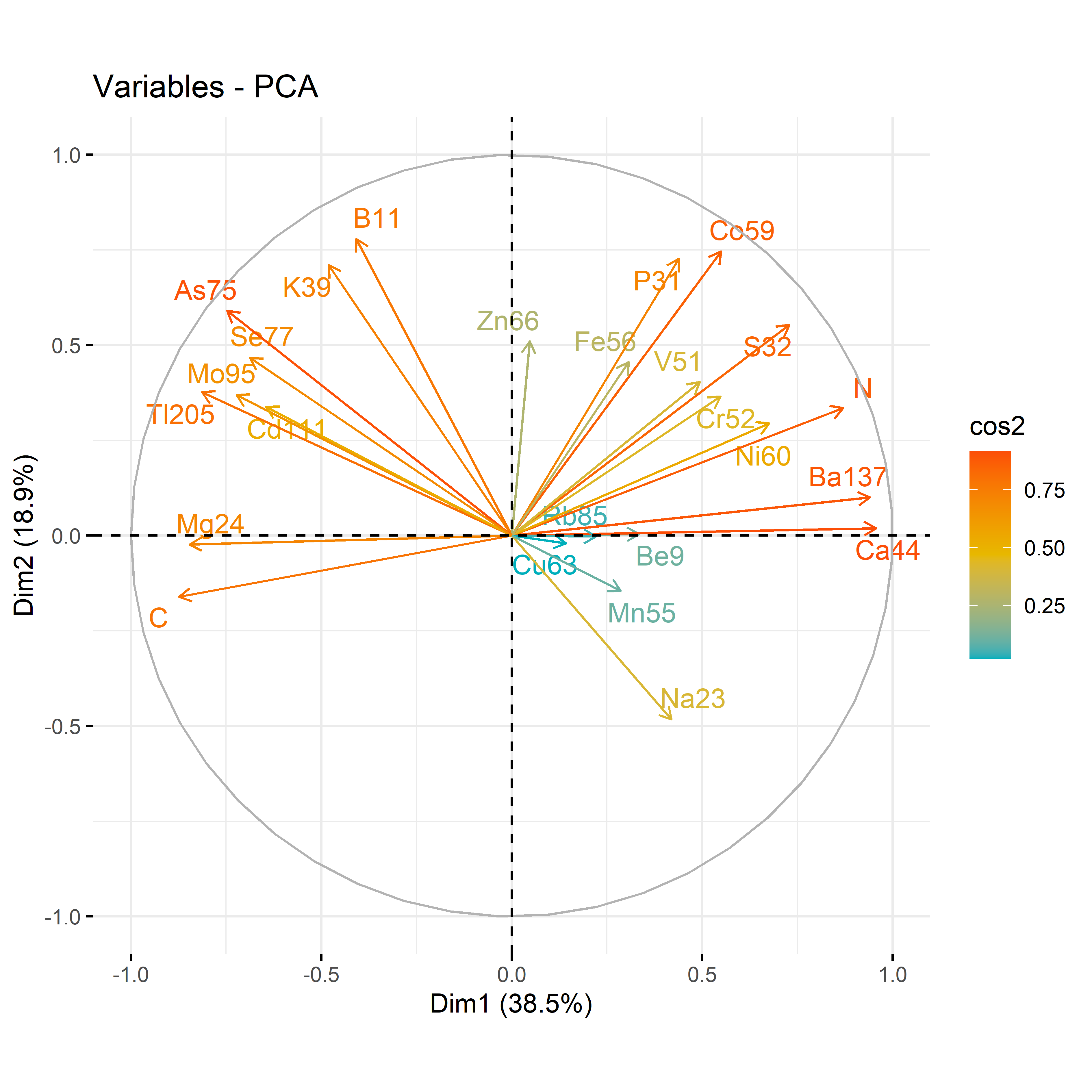
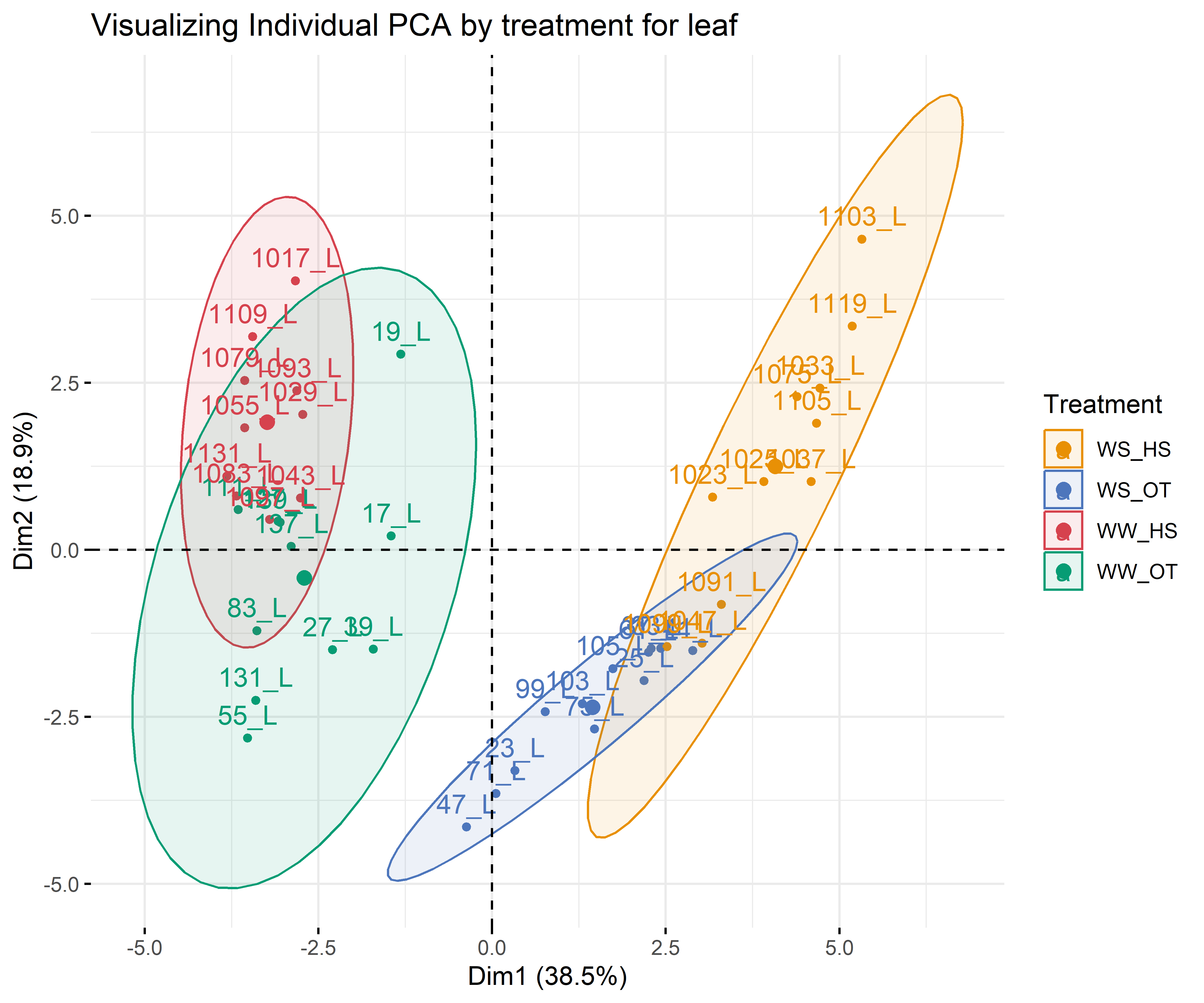
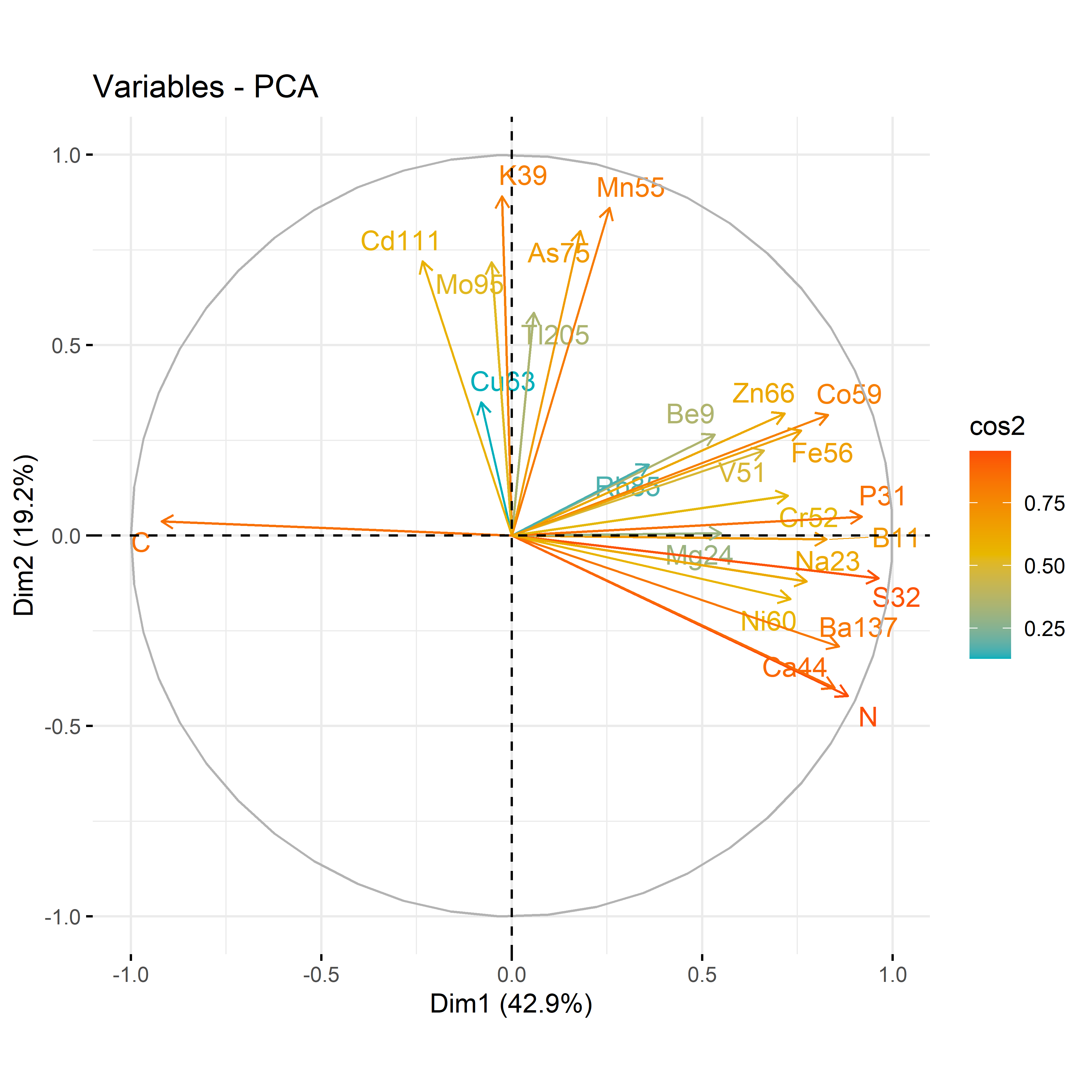
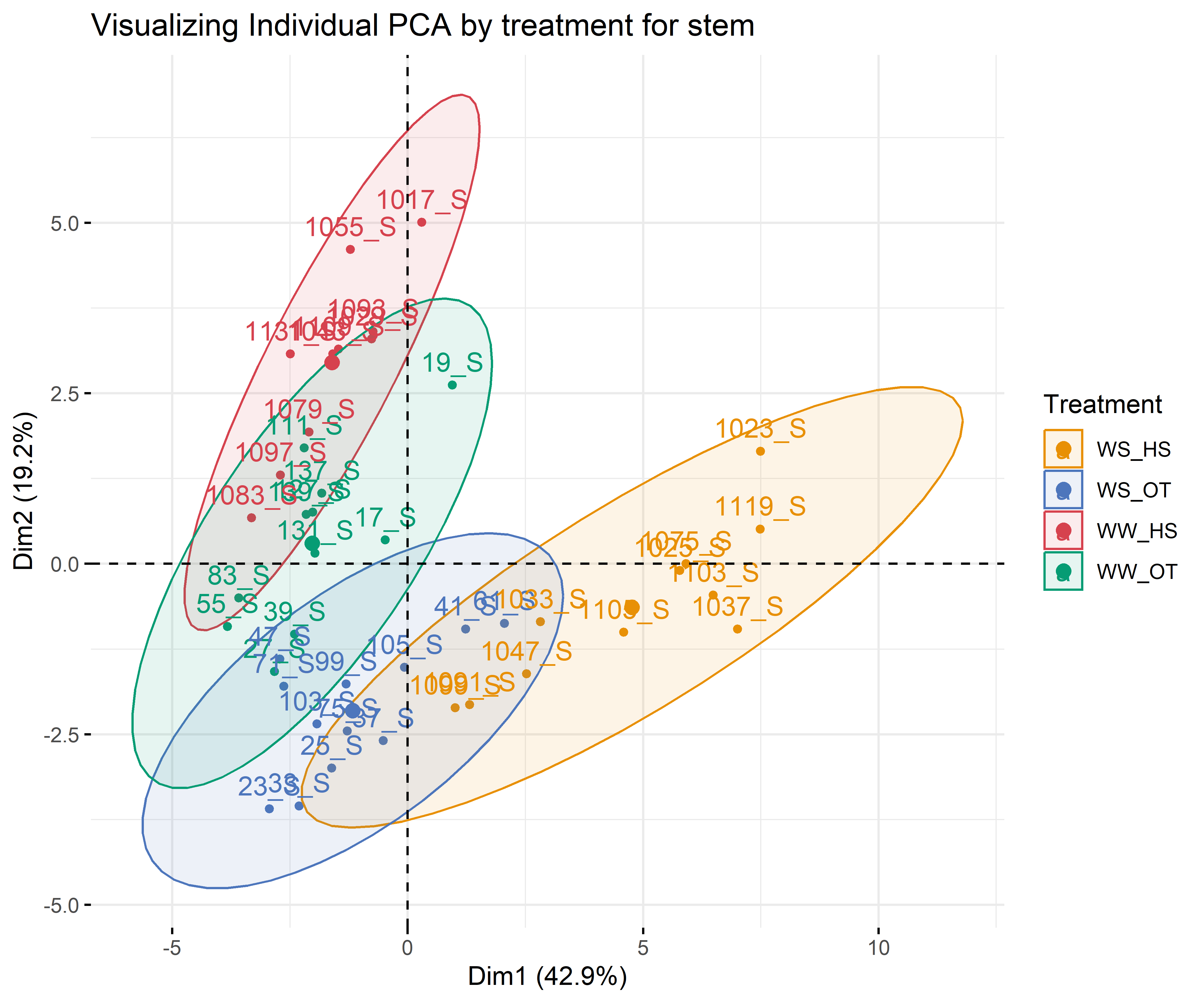
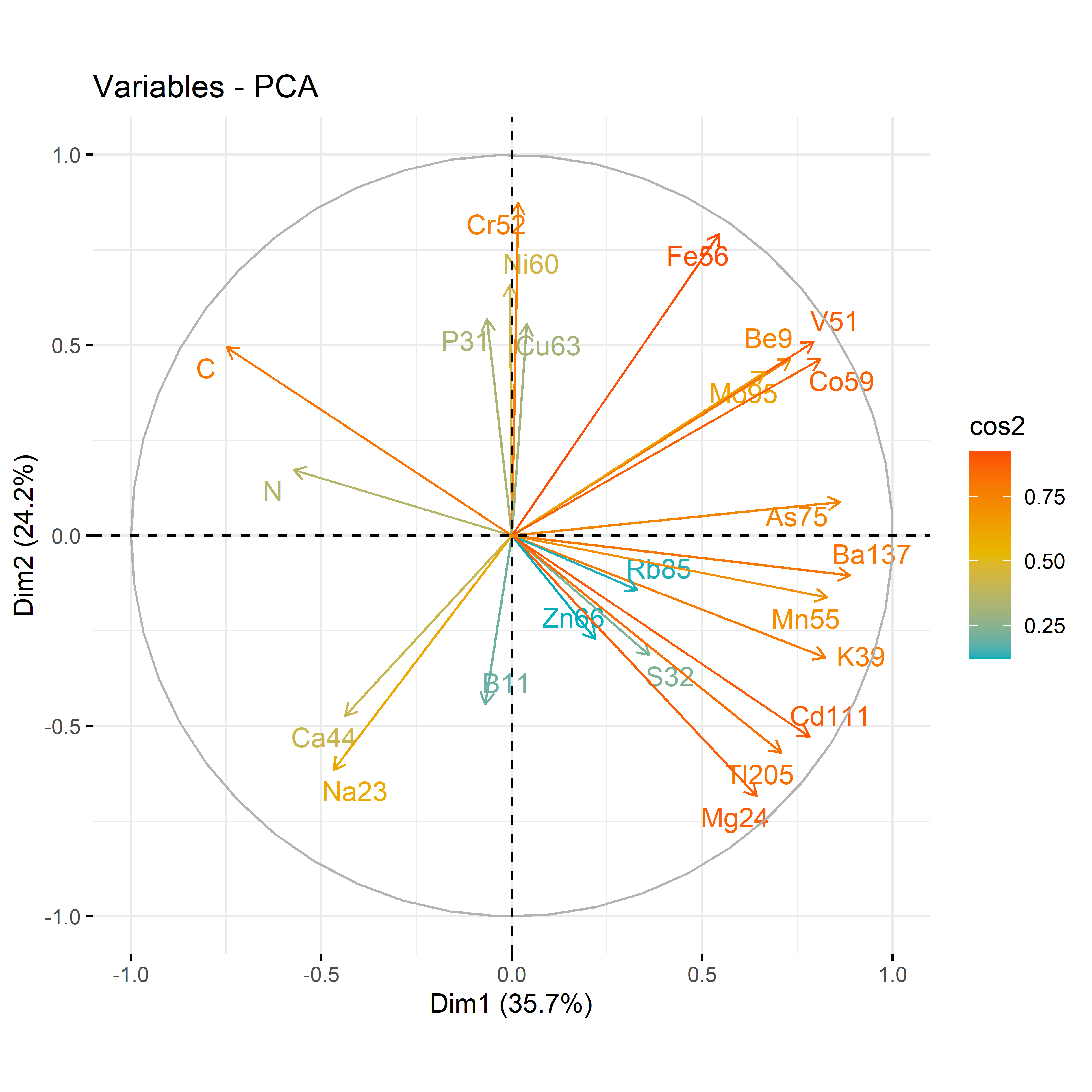
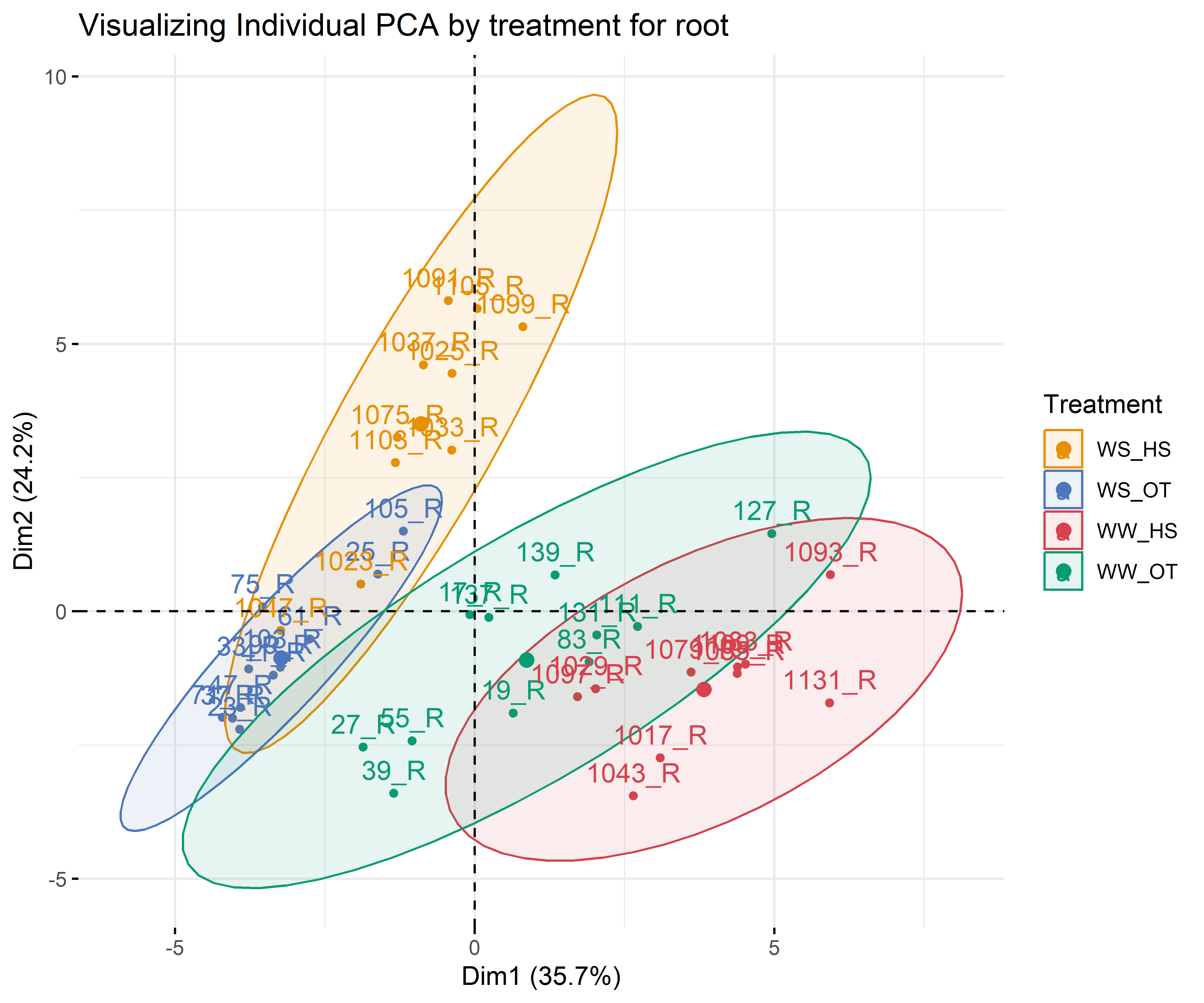
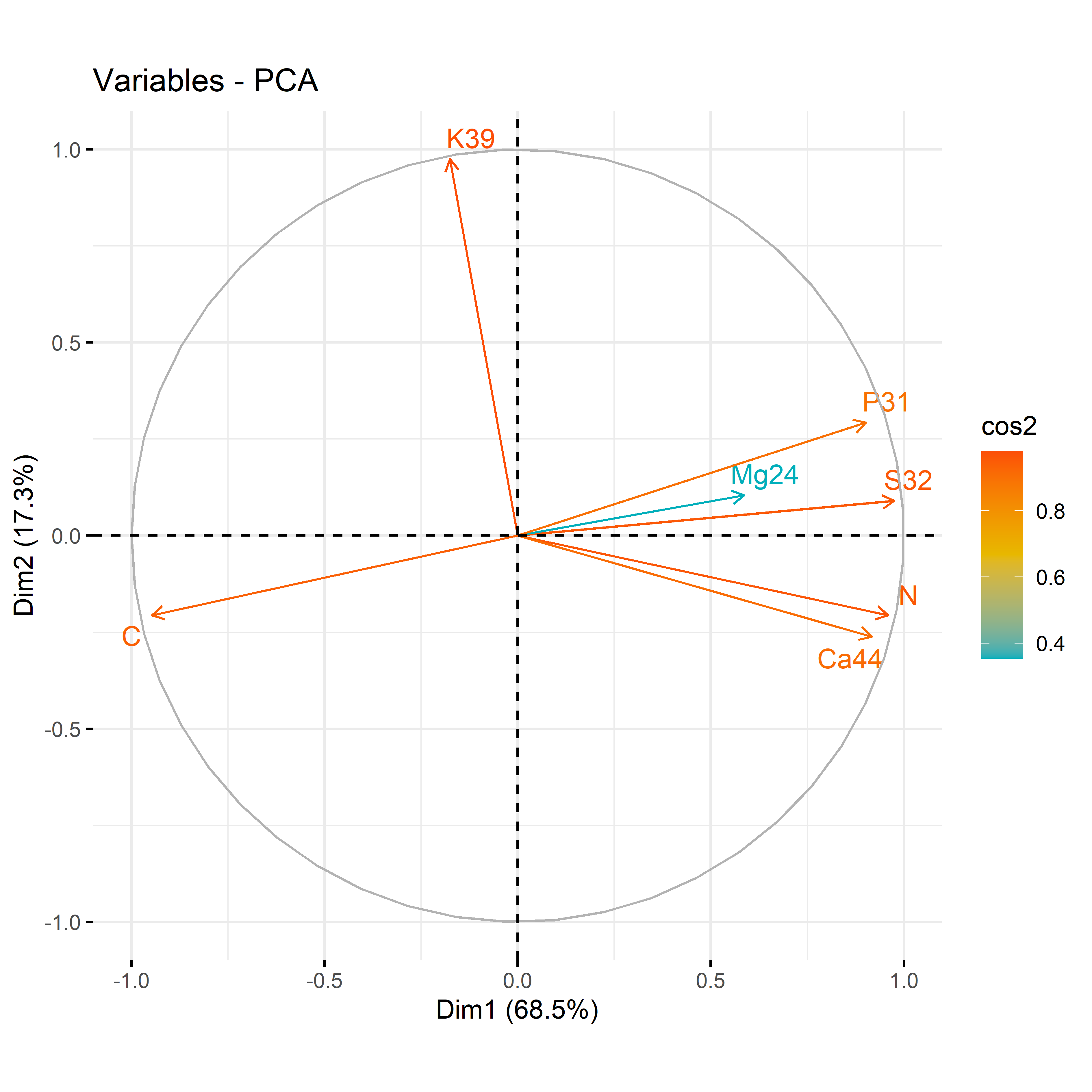
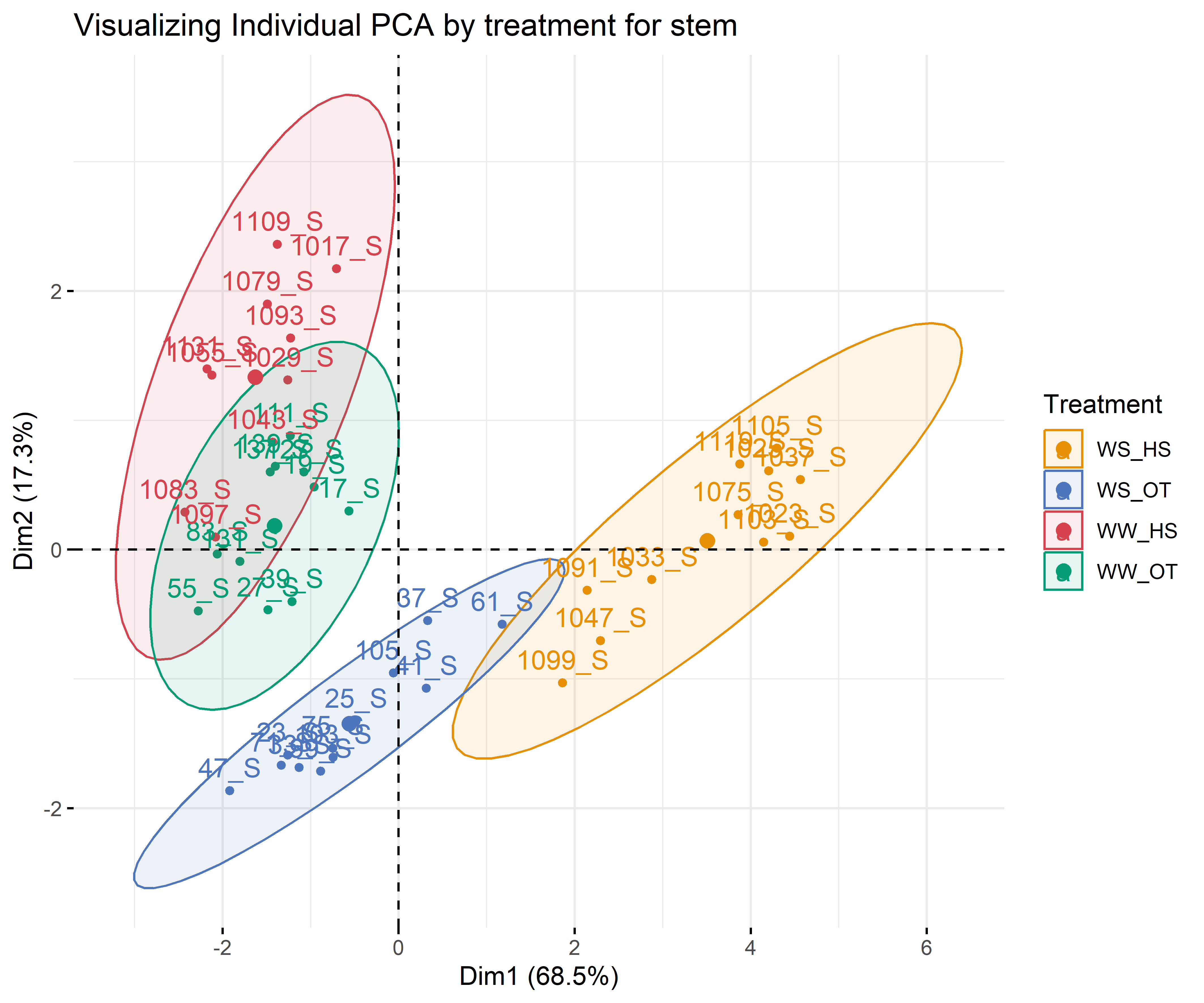
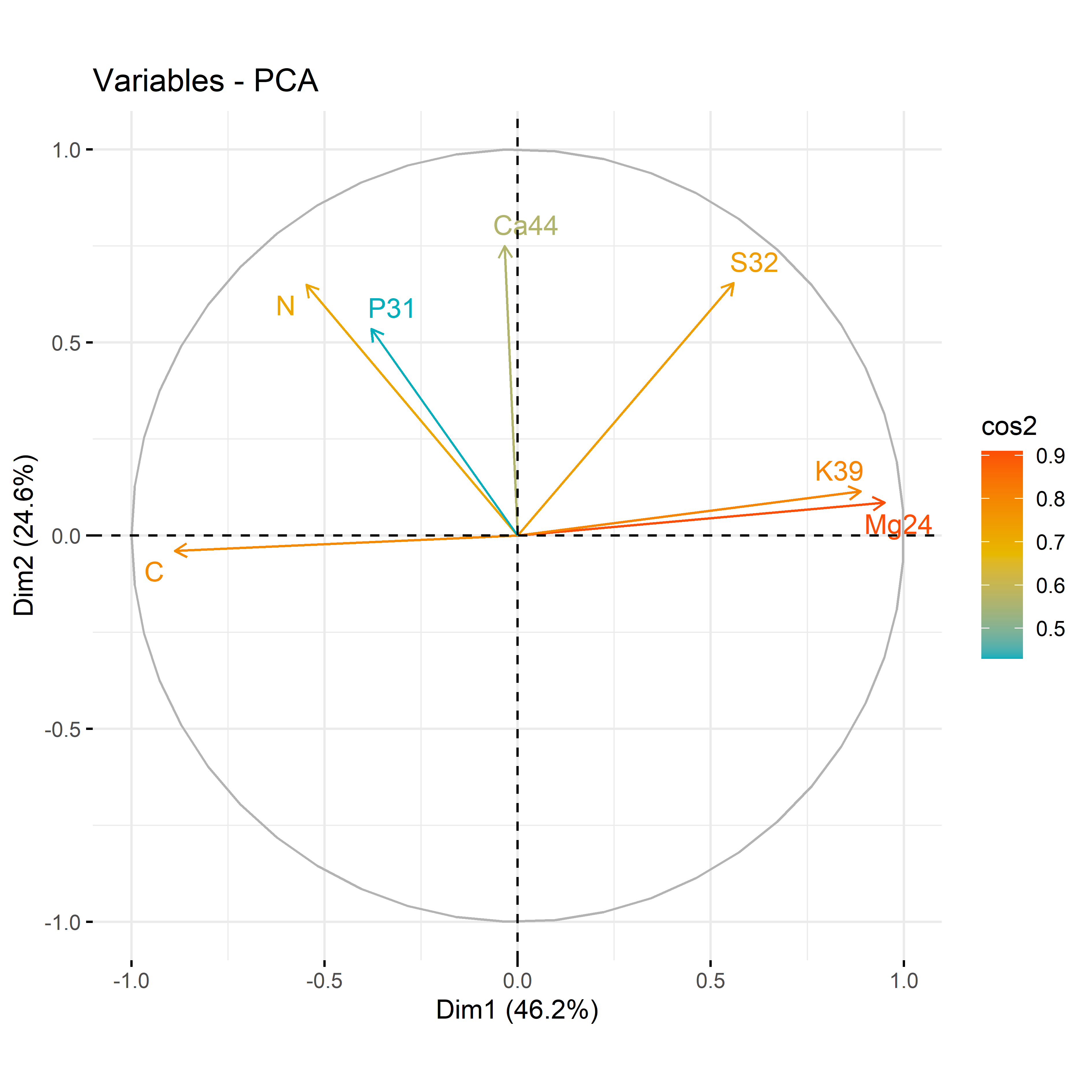
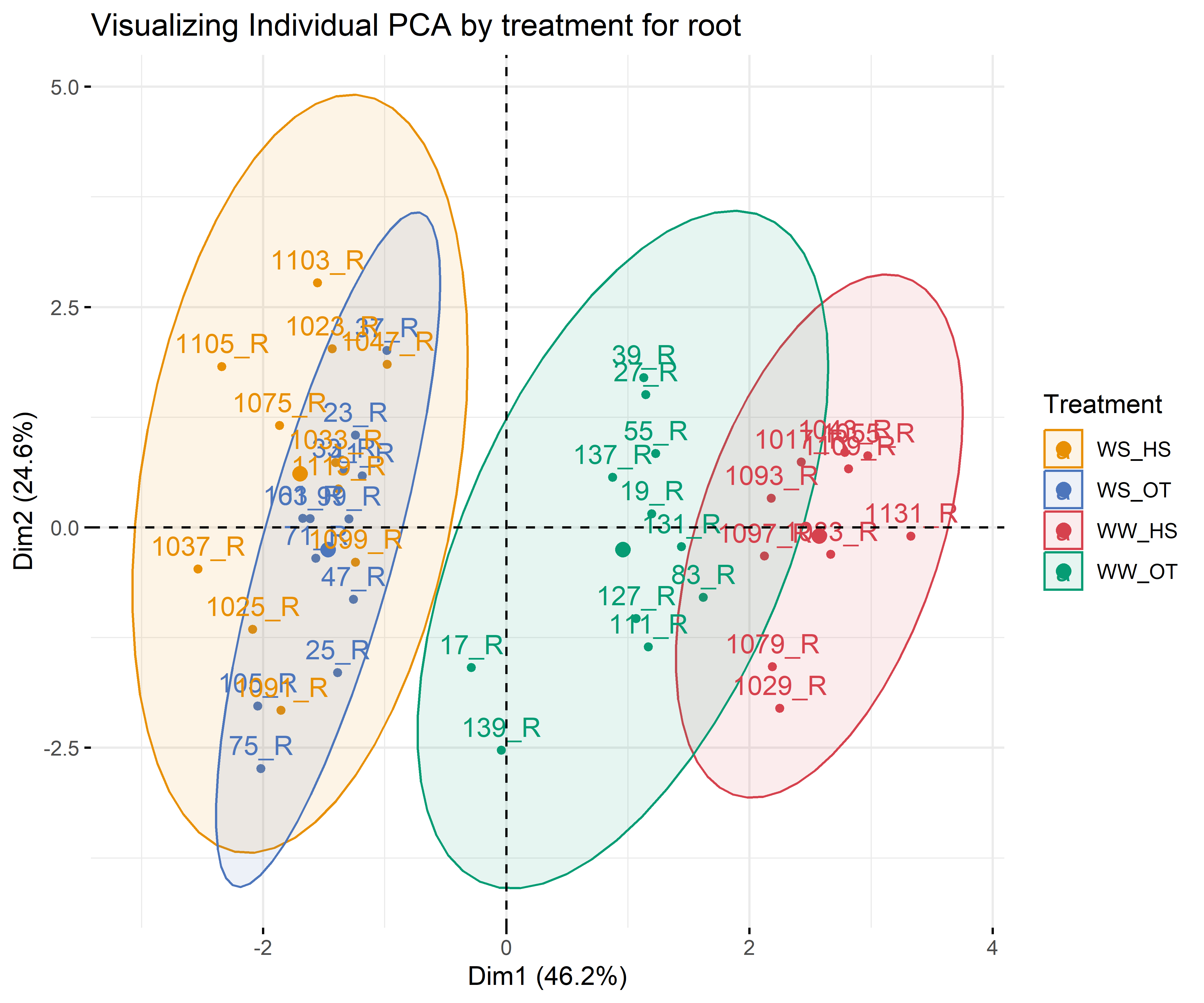
# leafdf_iono_leaf=df_ionomic_s_horizontal %>%filter(compartiment=="leaf")res_pca_iono_laef <-PCA(df_iono_leaf %>%as.data.frame() %>%column_to_rownames("id_sample"),quali.sup=1:3, graph = T)fviz_eig(res_pca_iono_laef, addlabels =TRUE, ylim =c(0, 50))var <-get_pca_var(res_pca_iono_laef)corrplot(var$cos2, is.corr=FALSE)png(here::here(paste0("report/iono/plot/ACP_var_by_treatment_for_leaf.png")), width =16, height =16, units ='cm', res =600)fviz_pca_var(res_pca_iono_laef, col.var ="cos2",gradient.cols =c("#00AFBB", "#E7B800", "#FC4E07"),repel =TRUE# Avoids text overlap)dev.off()png(here::here(paste0("report/iono/plot/ACP_by_treatment_for_leaf.png")), width =18, height =15, units ='cm', res =600)PCA_compartment<-fviz_pca_ind(res_pca_iono_laef,# geom.ind = "point", # Shows points only (not text)pointshape =20,pointsize =2,col.ind = df_ionomic_s_horizontal %>%filter(compartiment=="leaf") %>%mutate(climat_condition=substr(condition, 5, 9)) %>%pull(climat_condition), # colorer by groupspalett=c(climate_pallet),addEllipses = T, # Concentration ellipseslegend.title ="Treatment", ellipse.level =0.95,ellipse.type =c("norm"),)+ggtitle("Visualizing Individual PCA by treatment for leaf")PCA_compartmentdev.off()# stemdf_iono_stem=df_ionomic_s_horizontal %>%filter(compartiment=="stem") %>%dplyr::select(-Se77)res_pca_iono_stem <-PCA(df_iono_stem %>%as.data.frame() %>%column_to_rownames("id_sample"),quali.sup=1:3, graph = T)fviz_eig(res_pca_iono_stem, addlabels =TRUE, ylim =c(0, 50))var <-get_pca_var(res_pca_iono_stem)corrplot(var$cos2, is.corr=FALSE)png(here::here(paste0("report/iono/plot/ACP_var_by_treatment_for_stem.png")), width =16, height =16, units ='cm', res =600)fviz_pca_var(res_pca_iono_stem, col.var ="cos2",gradient.cols =c("#00AFBB", "#E7B800", "#FC4E07"),repel =TRUE# Avoids text overlap)dev.off()png(here::here(paste0("report/iono/plot/ACP_by_treatment_for_stem.png")), width =18, height =15, units ='cm', res =600)PCA_compartment<-fviz_pca_ind(res_pca_iono_stem,# geom.ind = "point", # Shows points only (not text)pointshape =20,pointsize =2,col.ind = df_ionomic_s_horizontal %>%filter(compartiment=="stem")%>%dplyr::select(-Se77) %>%mutate(climat_condition=substr(condition, 5, 9)) %>%pull(climat_condition), # colorer by groupspalett=c(climate_pallet),addEllipses = T, # Concentration ellipseslegend.title ="Treatment", ellipse.level =0.95,ellipse.type =c("norm"),)+ggtitle("Visualizing Individual PCA by treatment for stem")PCA_compartmentdev.off()# rootdf_iono_root=df_ionomic_s_horizontal %>%filter(compartiment=="root") %>% dplyr::select(-Se77) %>%filter(id_sample!="1119_R")res_pca_iono_root <-PCA(df_iono_root %>%as.data.frame() %>%column_to_rownames("id_sample"),quali.sup=1:3, graph = T)fviz_eig(res_pca_iono_root, addlabels =TRUE, ylim =c(0, 50))var <-get_pca_var(res_pca_iono_root)corrplot(var$cos2, is.corr=FALSE)png(here::here(paste0("report/iono/plot/ACP_var_by_treatment_for_root.png")), width =16, height =16, units ='cm', res =600)fviz_pca_var(res_pca_iono_root, col.var ="cos2",gradient.cols =c("#00AFBB", "#E7B800", "#FC4E07"),repel =TRUE# Avoids text overlap)dev.off()png(here::here(paste0("report/iono/plot/ACP_by_treatment_for_root.png")), width =18, height =15, units ='cm', res =600)PCA_compartment<-fviz_pca_ind(res_pca_iono_root,# geom.ind = "point", # Shows points only (not text)pointshape =20,pointsize =2,col.ind = df_ionomic_s_horizontal %>%filter(compartiment=="root") %>%mutate(climat_condition=substr(condition, 5, 9)) %>% dplyr::select(-Se77) %>%filter(id_sample!="1119_R")%>%pull(climat_condition), # colorer by groupspalett=c(climate_pallet),addEllipses = T, # Concentration ellipseslegend.title ="Treatment", ellipse.level =0.95,ellipse.type =c("norm"),)+ggtitle("Visualizing Individual PCA by treatment for root")PCA_compartmentdev.off()
12.3.3 For each compartment and only for macroelement
Code
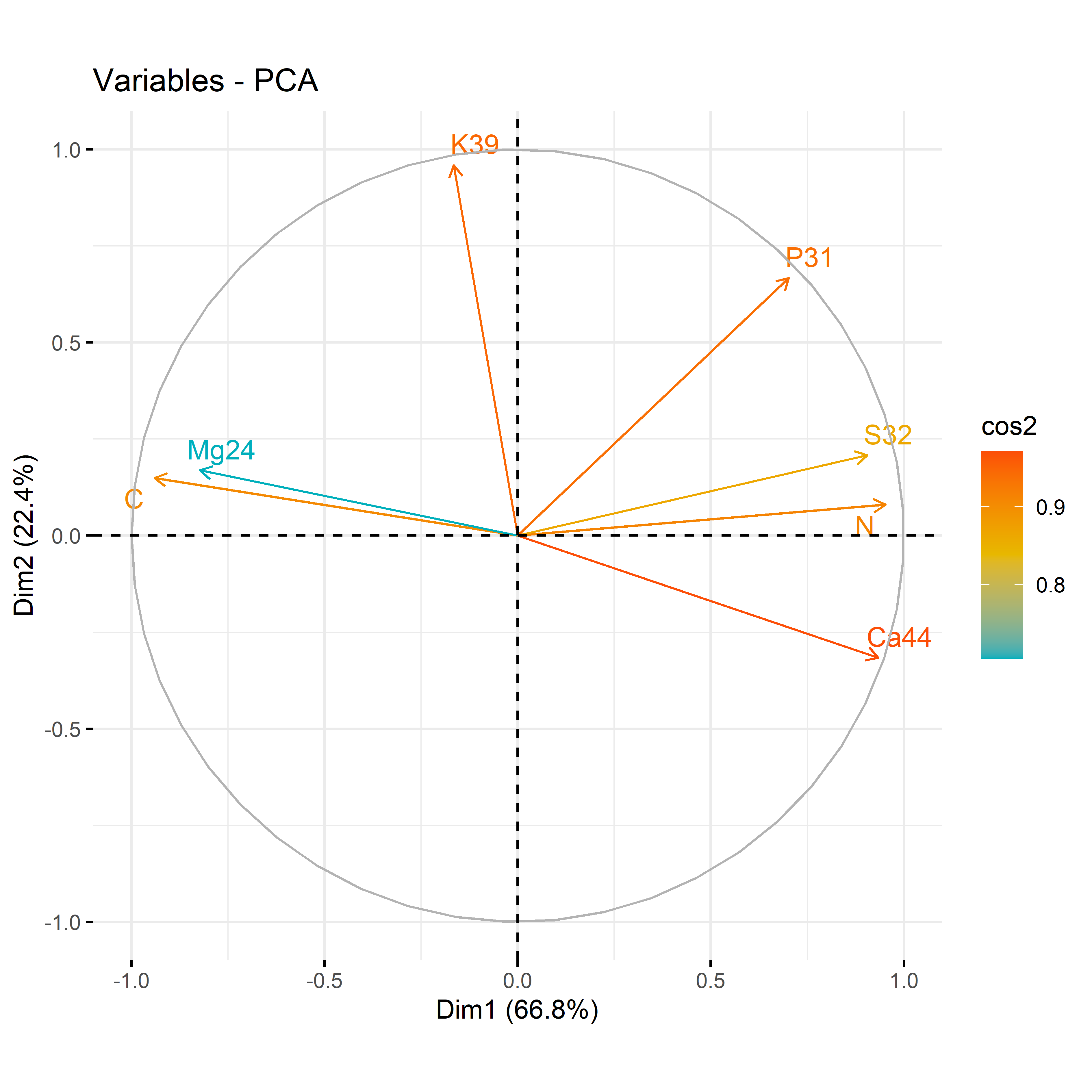
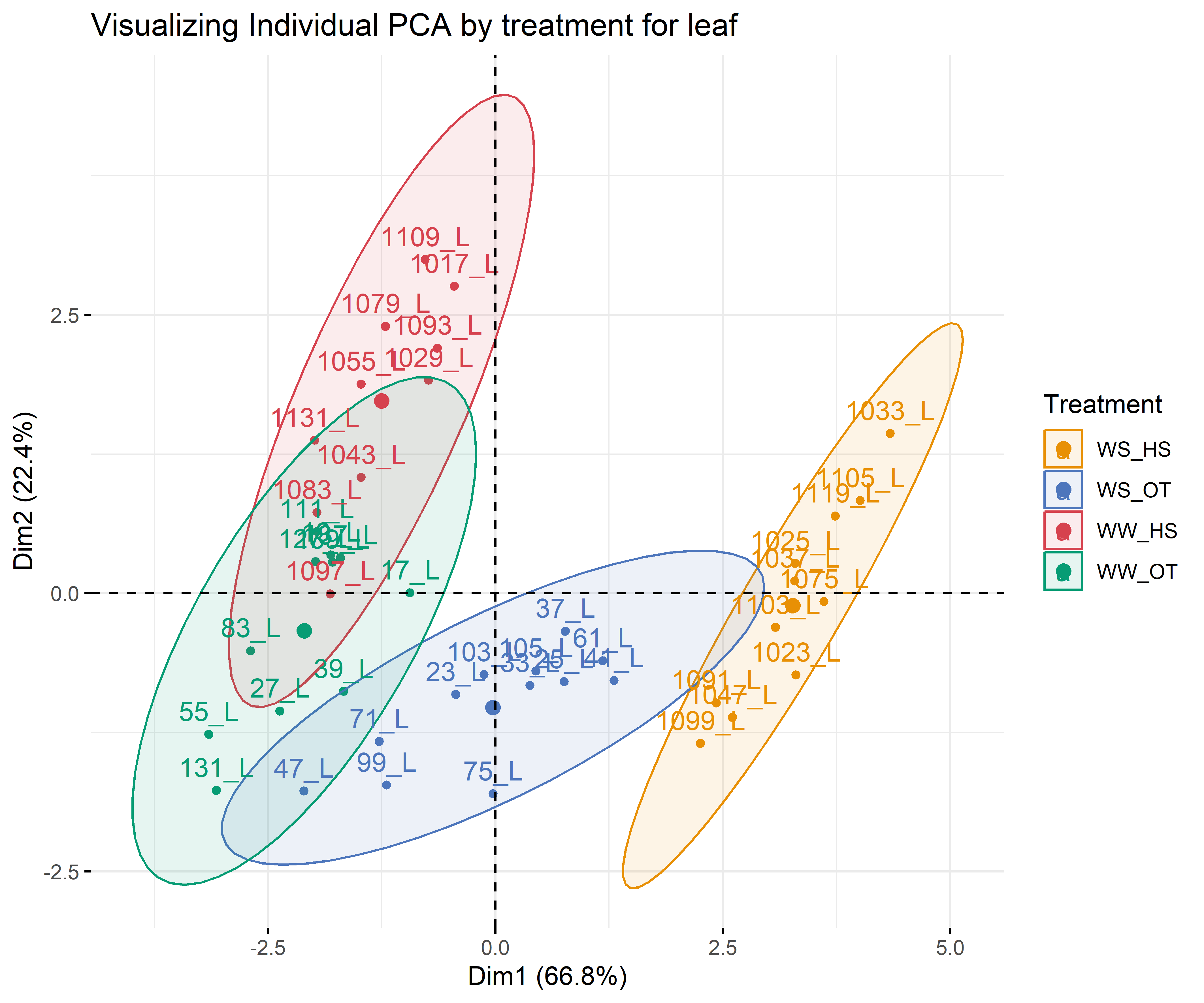
# leafdf_iono_leaf=df_ionomic_s_horizontal %>%filter(compartiment=="leaf") %>% dplyr::select(id_sample,condition_organe,compartiment,condition,N,C,Ca44,S32,Mg24,K39,P31)res_pca_iono_laef <-PCA(df_iono_leaf %>%as.data.frame() %>%column_to_rownames("id_sample"),quali.sup=1:3, graph = T)fviz_eig(res_pca_iono_laef, addlabels =TRUE, ylim =c(0, 50))var <-get_pca_var(res_pca_iono_laef)corrplot(var$cos2, is.corr=FALSE)png(here::here(paste0("report/iono/plot/ACP_var_by_treatment_for_leaf_macro_element.png")), width =16, height =16, units ='cm', res =600)fviz_pca_var(res_pca_iono_laef, col.var ="cos2",gradient.cols =c("#00AFBB", "#E7B800", "#FC4E07"),repel =TRUE)dev.off()png(here::here(paste0("report/iono/plot/ACP_by_treatment_for_leaf_macro_element.png")), width =18, height =15, units ='cm', res =600)PCA_compartment<-fviz_pca_ind(res_pca_iono_laef,pointshape =20,pointsize =2,col.ind = df_ionomic_s_horizontal %>%filter(compartiment=="leaf") %>%mutate(climat_condition=substr(condition, 5, 9)) %>%pull(climat_condition), # colorer by groupspalett=c(climate_pallet),addEllipses = T, legend.title ="Treatment", ellipse.level =0.95,ellipse.type =c("norm"),)+ggtitle("Visualizing Individual PCA by treatment for leaf")PCA_compartmentdev.off()# stemdf_iono_stem=df_ionomic_s_horizontal %>%filter(compartiment=="stem") %>% dplyr::select(id_sample,condition_organe,compartiment,condition,N,C,Ca44,S32,Mg24,K39,P31)res_pca_iono_stem <-PCA(df_iono_stem %>%as.data.frame() %>%column_to_rownames("id_sample"),quali.sup=1:3, graph = T)fviz_eig(res_pca_iono_stem, addlabels =TRUE, ylim =c(0, 50))var <-get_pca_var(res_pca_iono_stem)corrplot(var$cos2, is.corr=FALSE)png(here::here(paste0("report/iono/plot/ACP_var_by_treatment_for_stem_macro_element.png")), width =16, height =16, units ='cm', res =600)fviz_pca_var(res_pca_iono_stem, col.var ="cos2",gradient.cols =c("#00AFBB", "#E7B800", "#FC4E07"),repel =TRUE)dev.off()png(here::here(paste0("report/iono/plot/ACP_by_treatment_for_stem_macro_element.png")), width =18, height =15, units ='cm', res =600)PCA_compartment<-fviz_pca_ind(res_pca_iono_stem,# geom.ind = "point", pointshape =20,pointsize =2,col.ind = df_ionomic_s_horizontal %>%filter(compartiment=="stem") %>%mutate(climat_condition=substr(condition, 5, 9)) %>%pull(climat_condition), # colorer by groupspalett=c(climate_pallet),addEllipses = T,legend.title ="Treatment", ellipse.level =0.95,ellipse.type =c("norm"),)+ggtitle("Visualizing Individual PCA by treatment for stem")PCA_compartmentdev.off()# rootdf_iono_root=df_ionomic_s_horizontal %>%filter(compartiment=="root") %>% dplyr::select(id_sample,condition_organe,compartiment,condition,N,C,Ca44,S32,Mg24,K39,P31)res_pca_iono_root <-PCA(df_iono_root %>%as.data.frame() %>%column_to_rownames("id_sample"),quali.sup=1:3, graph = T)fviz_eig(res_pca_iono_root, addlabels =TRUE, ylim =c(0, 50))var <-get_pca_var(res_pca_iono_root)corrplot(var$cos2, is.corr=FALSE)png(here::here(paste0("report/iono/plot/ACP_var_by_treatment_for_root_macro_element.png")), width =16, height =16, units ='cm', res =600)fviz_pca_var(res_pca_iono_root, col.var ="cos2",gradient.cols =c("#00AFBB", "#E7B800", "#FC4E07"),repel =TRUE# Évite le chevauchement de texte)dev.off()png(here::here(paste0("report/iono/plot/ACP_by_treatment_for_root_macro_element.png")), width =18, height =15, units ='cm', res =600)PCA_compartment<-fviz_pca_ind(res_pca_iono_root,# geom.ind = "point", pointshape =20,pointsize =2,col.ind = df_ionomic_s_horizontal %>%filter(compartiment=="root") %>%mutate(climat_condition=substr(condition, 5, 9)) %>%pull(climat_condition), # colorer by groupspalett=c(climate_pallet),addEllipses = T, legend.title ="Treatment", ellipse.level =0.95,ellipse.type =c("norm"),)+ggtitle("Visualizing Individual PCA by treatment for root")PCA_compartmentdev.off()
The aim here is just to see how the elements are remobilized in the plant as a function of conditions. Maybe there are differential allocation effects from roots to leaves or vice versa
df_iono=read.csv(here::here("data/iono/output/ionomic.csv")) %>%filter(recolte==2) %>%filter(compartiment=="stem") %>%mutate(across(c(genotype, water_condition, heat_condition), factor)) %>%mutate(water_condition=relevel(water_condition, "WW")) %>%mutate(heat_condition=relevel(heat_condition, "OT")) %>% dplyr::select(plant_num, condition, genotype, water_condition, heat_condition, compound, correct_concentration) %>%pivot_wider(names_from = compound, values_from = correct_concentration) %>%drop_na(S32, N) %>%mutate(S_N= S32/N)contrasts(df_iono$genotype) <- contr.sum # to say look at the big average only for genotype (juste an other representation)mod1=lm(formula = C ~ water_condition*heat_condition*genotype, data = df_iono %>%drop_na(S32, N),contrasts =list(genotype = MASS::contr.sdif))p_x<-ggcoef_model(mod1) # ; p_xggsave(here::here("report/iono/plot/ggcoef_model_1.svg"),p_x)
A criterion must be defined to determine the quality of a model. One of the most widely used is the Akaike Information Criterion or AIC. It is a compromise between the number of degrees of freedom (e.g. the number of coefficients in the model) we wish to minimize and the explained variance we wish to maximize (the likelihood).
The AIC resuls for this first model is 900.95
The step() function selects the best model using a top-down step-by-step procedure based on AIC minimization. The function displays the various selection steps on the screen and returns the final model.
The AIC resuls for this second model is 895.7
Display performance indicators and the regression results


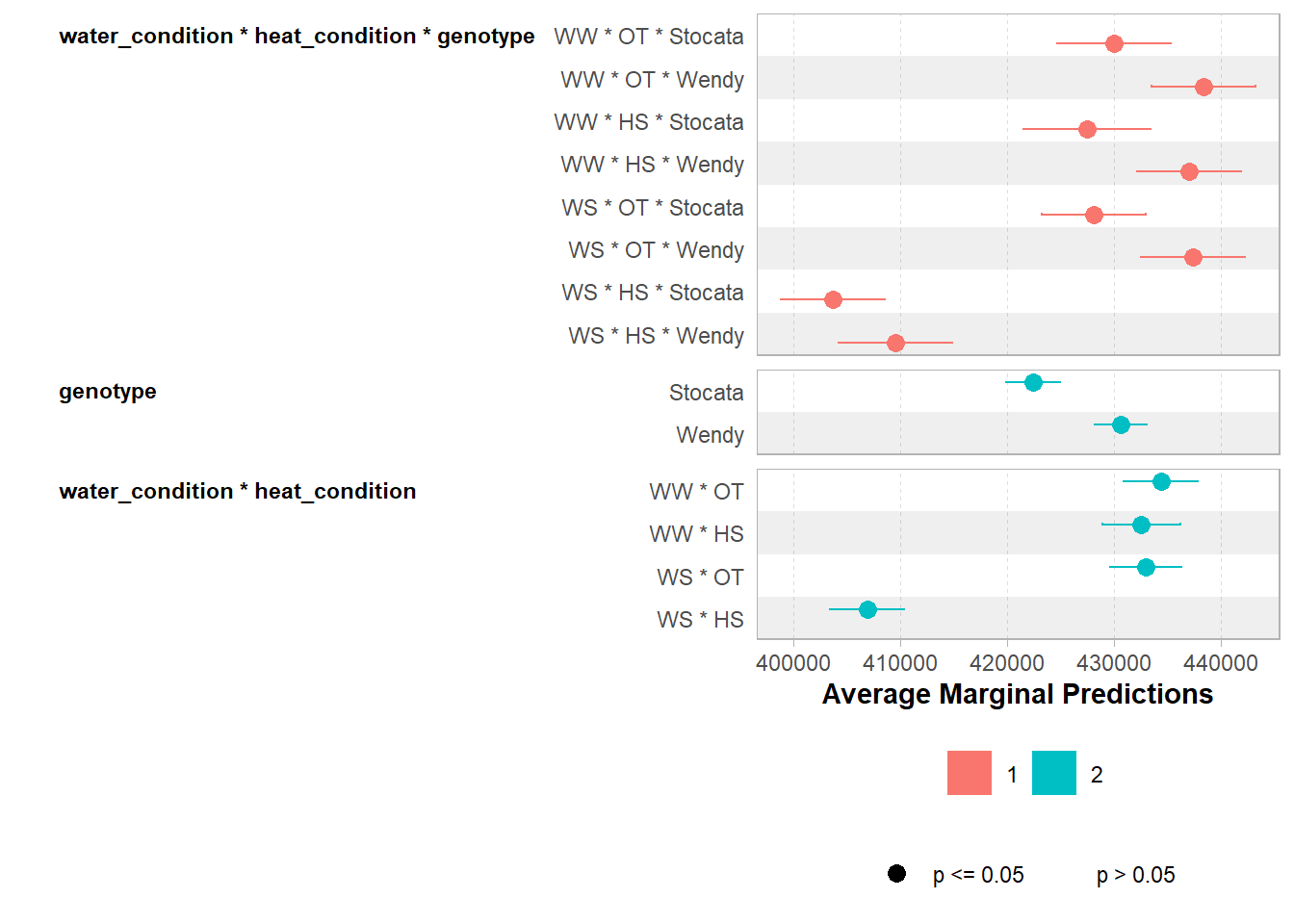
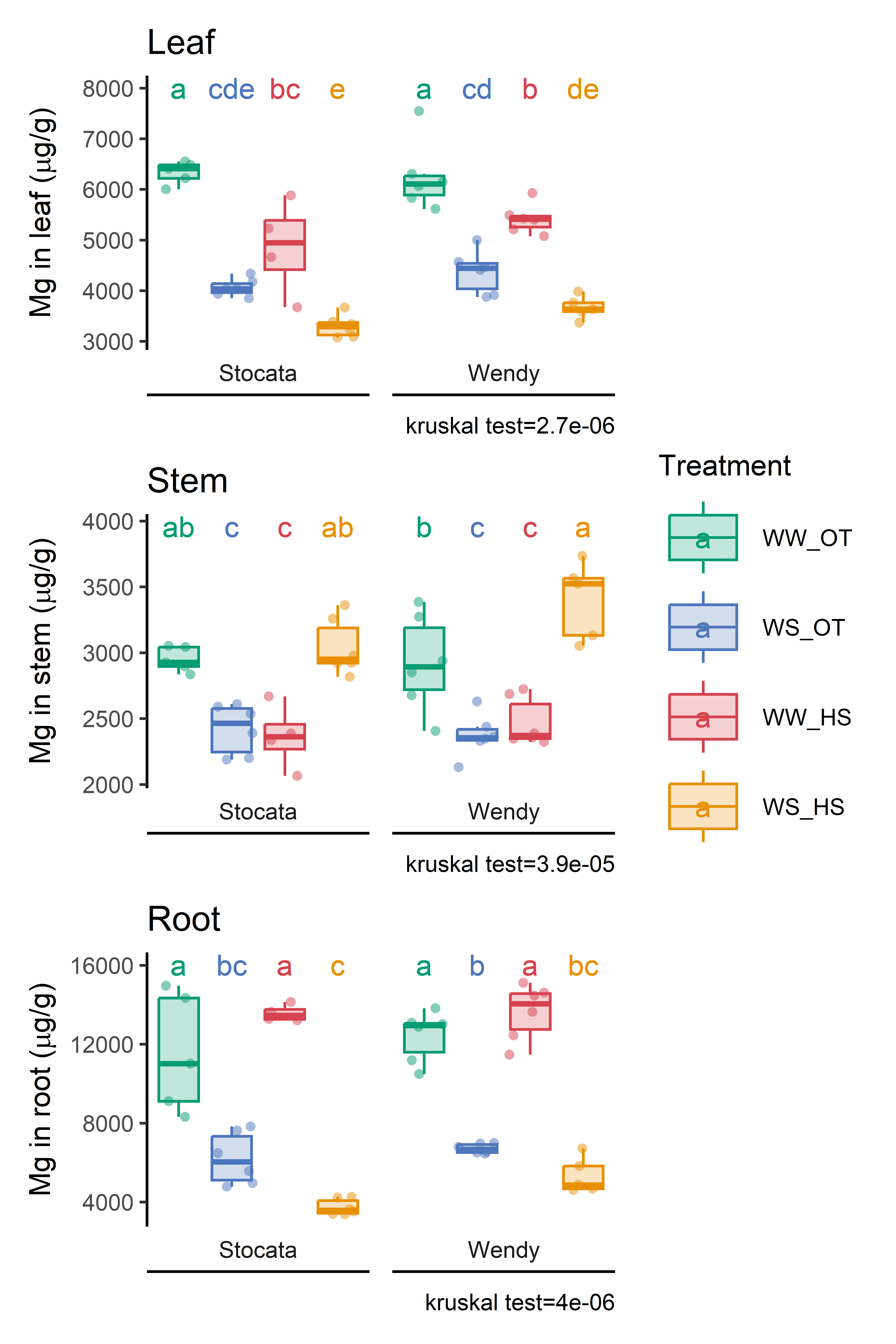 Show Mg content for reviewer