#package ----library(tidyr)library(readxl)library(ggplot2)library(plotly)library(vroom)library(ggExtra)library(stringr)library(gt)library(dplyr)library(gt) #gramar tablelibrary(DT)library(tidyverse)library(here)library(kableExtra)plant_info=read_excel(here::here("data/plant_information.xlsx"))source(here::here("src/function/root_architecture/data_importation_root_architecture.R")) #data importation for root tips, machin learning or anglesource(here::here("src/function/stat_function/stat_analysis_main.R")) # for make plot # cosmeticsclimate_pallet=read_excel(here::here("data/color_palette.xlsm")) %>%filter(set =="climat_condition") %>% dplyr::select(color, treatment) %>%pull(color) %>%setNames(read_excel(here::here("data/color_palette.xlsm")) %>%filter(set =="climat_condition") %>%pull(treatment) )
7.1 Contexte
Seedlings were grown in RhizoTubes® filled with sandy soil, allowing the visualization of the root system Jeudy et al. (2016)
Figure 7.1: The RhizoTube. The RhizoTube (a) is composed of concentrical tubes (an outer transparent PMA tube, an inner inox tubes) tighted together to the bottom and upper parts of RhizoTubes thanks to an axe, a bottom bolt and an upper star shaped tighting piece (b). Nutri solution supplied by the top (b) of the RhizoTube flows within the RhizoTube to the substrate, filled in between the inner tube and a membrane, permeable to nutrients, water and microbes but not to plant roots. This membrane has been tinted in blue with physiological inert ink to avoid any interference with plant growth. The seeds are placed at the top of the RhizoTube (c) and the plant root grows in its root propagation area (c) defined as the space between the outer transparent tube and the membrane. RhizoTubes are installed on conveyors thanks to a special adapted basis, which contains a unique RFID per Rhizotubes. From Jeudy et al. (2016).
The purpose of this script is to synthesize all my architecture data, to write all the import steps with the multiple specificities of the import. At the end, I will generate csv files of root architecture. Each file corresponds to a different type of data. For example, data per plant, per depth in the rhizotube etc.
7.2 Data importation
The raw data from machine learning is not included in this book because the file is over 9 GB.
7.2.1 For machine learning segmentation
Code
#add/ extracte info to/ from data warning !!! is too slowinput_folder="result_v3bis"input_folder="results_v3"input_folder="result_v3_for_skull"input_folder="result_v4"input_folder="result_v5"input_folder_version="result_soybean_v6"#!!!!!!!!!!!!!!!!!!!!!!!!!#data_importation_root_architecture(input_folder)data_importation_root_architecture_v2(input_folder_version)#!!!!!!!!!!!!!!!!!!!!!!!!!ggplot(data=df_global_archi_info, aes(x=shooting_date, y=volume, col= climat_condition))+geom_point()
I’ve gone through this stage, and here are the results.
Code
input_folder_version="result_soybean_v6"root_archi=read.csv(here::here(paste0("data/root/",input_folder_version,"/root_architecture_co_",input_folder_version,".csv"))) %>%# import data previously createmutate(taskid=substr(taskid,1,nchar(taskid))) %>%mutate(condition=factor(condition,levels=c("Sto_WW_OT","Sto_WW_HS","Sto_WS_OT","Sto_WS_HS","Wen_WW_OT","Wen_WW_HS","Wen_WS_OT","Wen_WS_HS"))) %>%mutate(plant_num_taskid=paste(sep="_",plant_num,taskid)) %>%filter(is.na(induct_error_root_architecture))
Next step, cleaning of the data root architecture for verficiation number of data
7.2.2 Verification if have all the plant or duplicate results
Code
list_taskid_post_analyse=levels(as.factor(root_archi_net$taskid))#source(here::here("xp1_analyse/rapport/root_architecture/function/verif_nb_data.R")) #may be i need to verify this data
I have some wird result why ? Because i have some duplicate value
Code
root_archi_net %>%filter(taskid==28480) %>%filter(plant_num==102) #OK, no problem, the same 102 in duplicate. df_verif=root_archi_net %>%filter(taskid==28504) #for taskid 28504 the 1099 is missingdf_verif=root_archi_net %>%filter(taskid==28510) %>%filter(plant_num%in%c(105, 105 , 106 ,107 ,108 ,109,110)) #OK, no problem, same dublicats.df_verif=root_archi_net %>%filter(taskid==28525) %>%filter(plant_num%in%c(103,104)) #OK, no problem, same dublicats.df_verif=root_archi_net %>%filter(taskid==28627) %>%filter(plant_num%in%c(103,104)) #OK, no problem, same dublicats.df_verif=root_archi_net %>%filter(taskid==28752) %>%filter(plant_num%in%c(103,104)) #OK, no problem, same dublicats.
Then I delete the possible duplicates by using a taskid plant num column. I checked manually that I had the same data
Import and refocus all root with function clean_csv_root_tips
Code
#can be easier if I start with all the root architecture data and then add the information. #collect all coo coo_root_tips_merged=as.data.frame(matrix(data=NA, ncol =6,nrow =0)) ; colnames(coo_root_tips_merged)=c("taskid","Label" , "XM" ,"YM", "X_calc", "Y_calc")for (taskid in taskids){ name_folder=paste0("csv_pointes_",taskid) path=here::here(paste0(path_input_data,name_folder)) file_names=list.files(path,pattern="csv")for (i in1:length(file_names)){ coo_root_tips_merged=rbind(coo_root_tips_merged,clean_csv_root_tips(file_names[i])) }}#extract date and timecoo_root_tips_merged$date_shooting=str_split_i(coo_root_tips_merged$Label,"_",16)coo_root_tips_merged$time_shooting=gsub(str_split_i(coo_root_tips_merged$Label,"_",17), pattern=".png$", replacement="")
Merge with plant info
Code
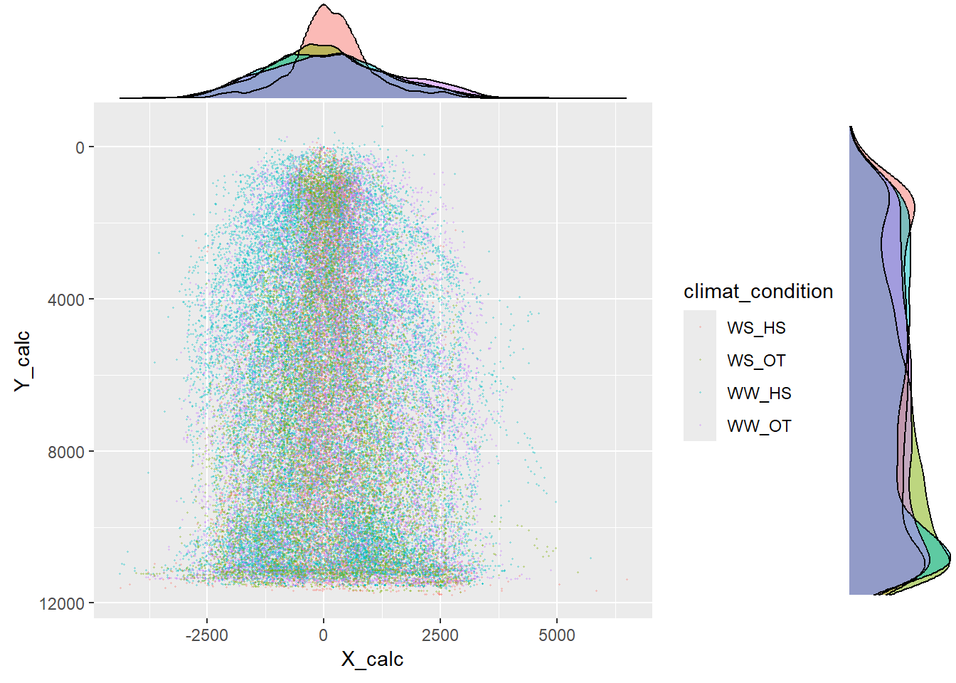
#merge with df plant_info for all data coo_root_tips_merged=merge(coo_root_tips_merged, plant_info %>% dplyr::select(plant_num, condition,genotype, water_condition, heat_condition), all=T, by="plant_num")coo_root_tips_merged$climat_condition=paste(sep="_",coo_root_tips_merged$water_condition,coo_root_tips_merged$heat_condition)#delet plant without root positioncoo_root_tips_select=coo_root_tips_merged %>%drop_na(Label)
160 plant are missing. So far we have counted 51839 root tips. From task:
28675 28688
Missing value:
integer(0)
7.2.4 For root angles
create function who check :
Check that the first line is a pivot. NAN for side and for small_root. ok
Check that each column has the same number of data (sometimes there is not the same number, happens in very rare cases because of the imagej macro) by using yes no in column small_root (again with coordinate)
Check that there are no problems during the import
Code
for (taskid in taskids){ name_folder=paste0("csv_angles_",taskid) path=here::here(paste0(path_input_data,name_folder)) file_names=list.files(path,pattern="csv")for (i in1:length(file_names)){check_csv_root_angle(file_names[i]) }}
Combine data
Code
coo_root_angle_merged=as.data.frame(matrix(data=NA, ncol =45,nrow =0))colnames(coo_root_angle_merged)=c("branching","side","small_root","Angle_ABC","Angle_CBD","XA","YA","XB","YB","XC","YC","XD","YD","XC2","YC2","XD2","YD2","AB","BC","BD","CD","BC2","BD2","C2D2","Angle_ABD", "Angle_ABC2" ,"Angle_C2BD2", "Label","Circle","Size_pixel","plant_num","taskid","XA_calc","YA_calc","XB_calc","YB_calc","XC_calc","YC_calc","XD_calc","YD_calc","XC2_calc","YC2_calc","XD2_calc","YD2_calc","namefile" )for (taskid in taskids){ name_folder=paste0("csv_angles_",taskid) path=here::here(paste0(path_input_data,name_folder)) file_names=list.files(path,pattern="csv")for (i in1:length(file_names)){# print(file_names[i]) coo_root_angle_merged=rbind(coo_root_angle_merged,combine_csv_root_angle(file_names[i])) }}#extract date and timecoo_root_angle_merged$date_shooting=str_split_i(coo_root_angle_merged$Label,"_",16)coo_root_angle_merged$time_shooting=gsub(str_split_i(coo_root_angle_merged$Label,"_",17), pattern=".png$", replacement="")
Merge with plant info
Code
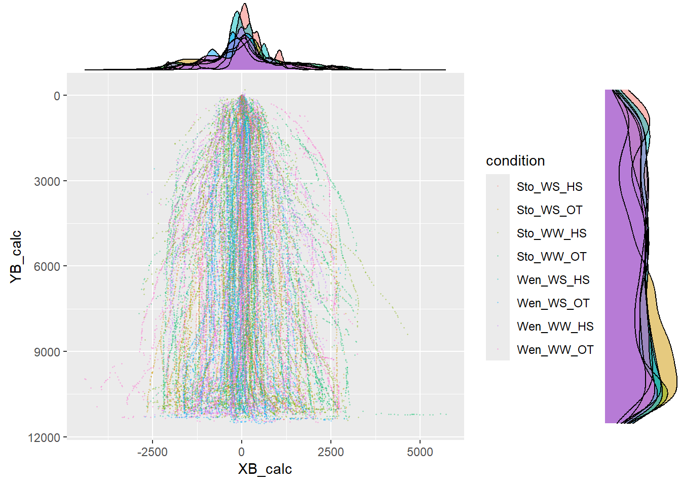
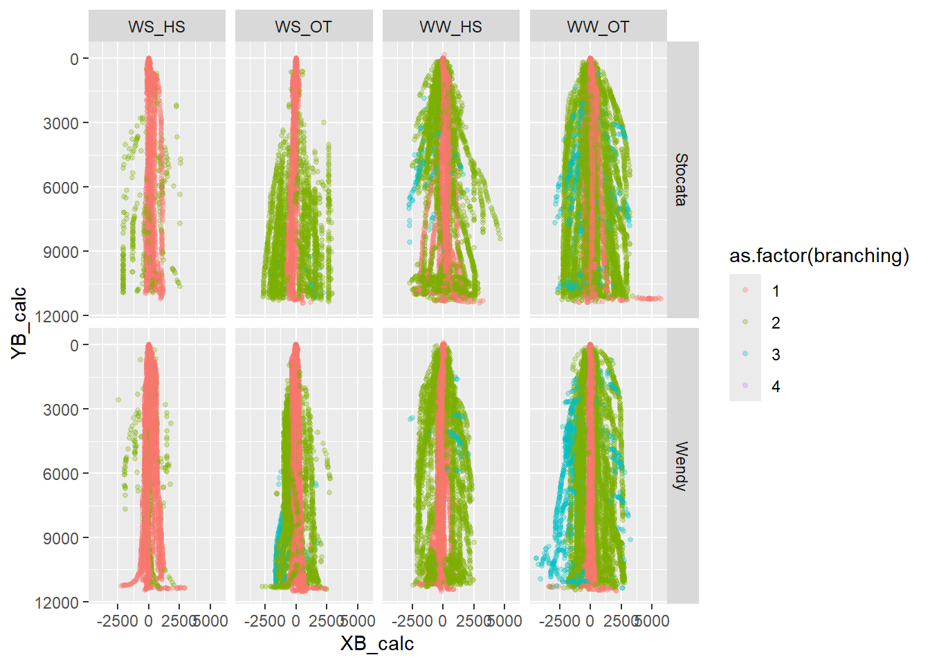
#merge with df plant_info for all data coo_root_angle_merged=merge(coo_root_angle_merged, plant_info %>% dplyr::select(plant_num, condition,genotype, water_condition, heat_condition,analyse_by_plant), all=T, by="plant_num")coo_root_angle_merged$climat_condition=paste(sep="_",coo_root_angle_merged$water_condition,coo_root_angle_merged$heat_condition)#delet plant without root positioncoo_root_angle_select=coo_root_angle_merged %>%drop_na(Label)
7.4.1 Combine for export all data frame by plant_num and date
Code
sum_tips_10000<-coo_root_tips_select %>%filter(YM<10000) %>%filter(plant_num!=1005) %>%#I have filtered so that I do not take the values below 10000 pixel (depending on the coordinates of YB). That is to say 41,66 cm of depth. group_by(condition,heat_condition,water_condition,genotype,plant_num,taskid) %>% dplyr::summarise(sum_nb_tips_10000 =n()) %>%mutate(condition=factor(condition,levels=c("Wen_WW_OT","Wen_WW_HS","Wen_WS_OT","Wen_WS_HS","Sto_WW_OT","Sto_WW_HS","Sto_WS_OT","Sto_WS_HS"))) %>%mutate(plant_num_taskid=paste(sep="_",plant_num, taskid)) %>%as.data.frame()#distance meandistance_mean_branching<-coo_root_angle_select %>%mutate(across( c(branching, plant_num), as.factor) ) %>%filter(YB<10000) %>%group_by(condition,heat_condition,water_condition,genotype,plant_num,branching,taskid) %>% dplyr::summarise(across(Angle_ABC:Angle_C2BD2, mean,na.rm=T,.names ="{.col}_mean")) %>%filter(branching !=4) %>%ungroup() %>%mutate(plant_num_taskid=paste(sep="_",plant_num, taskid)) %>%#dplyr::select(plant_num,condition, water_condition, heat_condition,branching,BC2) %>% pivot_wider(names_from="branching",values_from=c(Angle_ABC_mean:Angle_C2BD2_mean)) %>% dplyr::mutate(across(c(AB_mean_1:C2D2_mean_3), function(x) x*0.0042)) %>%as.data.frame() #sum (only for length)distance_sum_branching<-coo_root_angle_select %>%mutate(across( c(branching, plant_num), as.factor) ) %>%filter(YB<10000) %>%group_by(condition,heat_condition,water_condition,genotype,plant_num,branching,taskid) %>% dplyr::summarise(across(Angle_ABC:Angle_C2BD2, sum,na.rm=T,.names ="{.col}_sum")) %>%filter(branching !=4) %>%ungroup() %>%mutate(plant_num_taskid=paste(sep="_",plant_num, taskid)) %>%#dplyr::select(plant_num,condition, water_condition, heat_condition,branching,BC2) %>% pivot_wider(names_from="branching",values_from=c(Angle_ABC_sum:Angle_C2BD2_sum)) %>% dplyr::mutate(across(c(AB_sum_1:C2D2_sum_3), function(x) x*0.0042)) %>%as.data.frame() # nb ramification by branchingnb_branching_by_type_branching<-coo_root_angle_select %>%mutate(across( c(branching, plant_num), as.factor) ) %>%filter(YB<10000) %>%group_by(condition,heat_condition,water_condition,genotype,plant_num,branching,taskid) %>% dplyr::summarise(nb_ramif=n(),na.rm=T) %>%filter(branching !=4) %>%mutate(plant_num_taskid=paste(sep="_",plant_num, taskid)) %>%# dplyr::select(plant_num,condition, water_condition, heat_condition,branching,BC2) %>% pivot_wider(names_from="branching",values_from=nb_ramif,names_glue ="{.value}_{branching}"#rename automatically column ) %>%mutate_at(c(9:11), ~replace(., is.na(.), 0)) %>%#transform na to 0 dplyr::select(!na.rm) %>%mutate(sum_ramif_10000=nb_ramif_1+nb_ramif_2+nb_ramif_3) %>%as.data.frame()nb_tips_by_type_branching<-coo_root_angle_select %>%mutate(across( c(branching, plant_num), as.factor) ) %>%#filter(YC2<11000) %>% group_by(condition,heat_condition,water_condition,genotype,plant_num,branching,taskid) %>% dplyr::summarise(nb_tips_macro=n(),na.rm=T) %>%filter(branching !=4) %>%mutate(plant_num_taskid=paste(sep="_",plant_num, taskid)) %>%#dplyr::select(plant_num,condition, water_condition, heat_condition,branching,BC2) %>% pivot_wider(names_from="branching",values_from=nb_tips_macro,names_glue ="{.value}_{branching}"#rename automatically column ) %>%mutate_at(c(9:11), ~replace(., is.na(.), 0)) %>%#transform na to 0 dplyr::select(!na.rm) %>%mutate(sum_tips_macro=nb_tips_macro_1+nb_tips_macro_2+nb_tips_macro_3) %>%as.data.frame()# merge data by plant_num and taskiddf_global_macro<-merge(sum_tips_10000 %>% dplyr::select(plant_num_taskid,sum_nb_tips_10000), distance_mean_branching[,5:79] ,by="plant_num_taskid",all=T)distance_sum_branching=distance_sum_branching %>% dplyr::select(plant_num_taskid,"AB_sum_1","AB_sum_2" ,"AB_sum_3", "BC_sum_1" ,"BC_sum_2" ,"BC_sum_3", "BD_sum_1" , "BD_sum_2" , "BD_sum_3","CD_sum_1","CD_sum_2" ,"CD_sum_3","BC2_sum_1" ,"BC2_sum_2" ,"BC2_sum_3","BD2_sum_1" ,"BD2_sum_2", "BD2_sum_3","C2D2_sum_1" , "C2D2_sum_2" , "C2D2_sum_3")df_global_macro<-merge(df_global_macro, distance_sum_branching,by="plant_num_taskid",all=T)df_global_macro<-merge(df_global_macro,nb_branching_by_type_branching[,7:length(nb_branching_by_type_branching)],by="plant_num_taskid",all=T)df_global_macro<-merge(df_global_macro,nb_tips_by_type_branching[,7:length(nb_branching_by_type_branching)],by="plant_num_taskid",all=T)df_global_ra<-merge(root_archi, df_global_macro %>%select(!c(taskid,plant_num)),by="plant_num_taskid",all=T)
7.4.2 Add shoot architecture
My problem is that I had for primary key plant_num taskid. But for the stems I only have shooting date and plant num. I will have to recreate a second primary key but with shooting date. Do I have duplicate shooting date and plant_num (a plant photographed twice)
Code
#verif for stem and for roottest=read.csv(here::here("data/physio/output/result_convex_hull_hauteur_tige_analyse_v1_to_modif.csv")) %>%mutate(plant_num_shooting_date=paste(sep="_",plant_num,shooting_date)) %>%group_by(plant_num_shooting_date) %>%filter(n()>1)test=df_global_ra%>%mutate(plant_num_shooting_date=paste(sep="_",plant_num,shooting_date)) %>%group_by(plant_num_shooting_date) %>%filter(n()>1)
Remove all the information that are in root architecture (coming from plant_information) merge the two datasets and re-add the data
df_global_archi_info_resum<-read.csv(here::here(here::here("data/root/output/global_architecture_plant_shooting_date_taskid.csv"))) %>%filter(recolte %in%c(1,2)) %>%drop_na(condition) %>% dplyr::group_by(condition, recolte,plant_num) %>% dplyr::summarise(count=n()) %>% dplyr::group_by(condition, recolte) %>% dplyr::summarise(Mean=mean(count), Sum=sum(count)) %>%mutate(Mean=round(Mean)) %>%pivot_wider(names_from = recolte, values_from =c(Mean, Sum)) # mean(df_global_archi_info_resum$Sum_2)df_global_archi_info_resum %>% dplyr::select(condition, Mean_1, Sum_1, Mean_2, Sum_2) %>%mutate(across(everything(), ~as.character(.))) %>%mutate(across(everything(), ~tidyr::replace_na(., "-"))) %>%kbl(caption ="Mean number of images per rhizotube and total number of images per condition", col.names=c("Condition", "Mean number of image (different dates) by rhizotube for H1", "Total number of images for H1","Mean number of image (different dates) by rhizotube for H2", "Total number of images for H2"), digits =0) %>%kable_paper(full_width = F)
Mean number of images per rhizotube and total number of images per condition
Condition
Mean number of image (different dates) by rhizotube for H1
Total number of images for H1
Mean number of image (different dates) by rhizotube for H2
Total number of images for H2
Sto_WS_HS
-
-
12
300
Sto_WS_OT
-
-
12
338
Sto_WW_HS
-
-
11
350
Sto_WW_OT
4
50
12
372
Wen_WS_HS
-
-
11
318
Wen_WS_OT
-
-
12
338
Wen_WW_HS
-
-
12
382
Wen_WW_OT
4
50
12
386
Jeudy, Christian, Marielle Adrian, Christophe Baussard, Céline Bernard, Eric Bernaud, Virginie Bourion, Hughes Busset, et al. 2016. “RhizoTubes as a New Tool for High Throughput Imaging of Plant Root Development and Architecture: Test, Comparison with Pot Grown Plants and Validation.”Plant Methods, 4.993, 12 (1): 31. https://doi.org/10.1186/s13007-016-0131-9.
Source Code
---output: html_documenteditor_options: chunk_output_type: console---## Pre-processing of root architecture data {#sec-root_archicture}::: callout-tip## Code for analysing high-resolution images<a href="./python_code/Supporting_Information_7.py" title="Téléchargez le script Python"> <img src="python_code/python.ico" alt="Python" style="width: 24px; height: 24px;"/> Download the Python script here </a><a href="./macro_java_code/Supporting_Information_8.ijm" title="Téléchargez le script Python"> <img src="macro_java_code/imagej.ico" alt="ImageJ Macro" style="width: 24px; height: 24px;"/> Download the Macro (java) here (.ijm) and import in Fiji or ImageJ </a>:::```{r}#package ----library(tidyr)library(readxl)library(ggplot2)library(plotly)library(vroom)library(ggExtra)library(stringr)library(gt)library(dplyr)library(gt) #gramar tablelibrary(DT)library(tidyverse)library(here)library(kableExtra)plant_info=read_excel(here::here("data/plant_information.xlsx"))source(here::here("src/function/root_architecture/data_importation_root_architecture.R")) #data importation for root tips, machin learning or anglesource(here::here("src/function/stat_function/stat_analysis_main.R")) # for make plot # cosmeticsclimate_pallet=read_excel(here::here("data/color_palette.xlsm")) %>%filter(set =="climat_condition") %>% dplyr::select(color, treatment) %>%pull(color) %>%setNames(read_excel(here::here("data/color_palette.xlsm")) %>%filter(set =="climat_condition") %>%pull(treatment) )```## ContexteSeedlings were grown in RhizoTubes® filled with sandy soil, allowing the visualization of the root system [@jeudy2016](see @fig-rhizotube)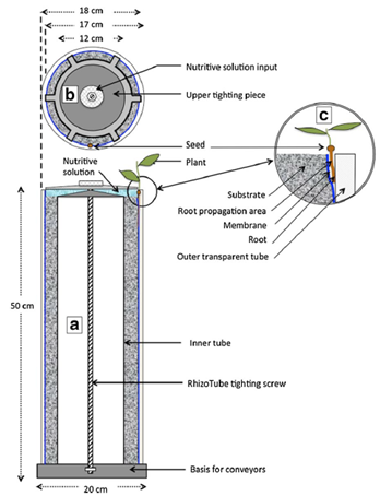{#fig-rhizotube}The purpose of this script is to synthesize **all my architecture data**, to write all the import steps with the multiple specificities of the import. At the end, I will generate csv files of root architecture. Each file corresponds to a different type of data. For example, data per plant, per depth in the rhizotube etc.## Data importation::: callout-warning## The raw data from machine learning is not included in this book because the file is over 9 GB.:::### For machine learning segmentation```{r, ImportMachineLearningPart1,eval=F}#add/ extracte info to/ from data warning !!! is too slowinput_folder="result_v3bis"input_folder="results_v3"input_folder="result_v3_for_skull"input_folder="result_v4"input_folder="result_v5"input_folder_version="result_soybean_v6" #!!!!!!!!!!!!!!!!!!!!!!!!!#data_importation_root_architecture(input_folder)data_importation_root_architecture_v2(input_folder_version)#!!!!!!!!!!!!!!!!!!!!!!!!!ggplot(data=df_global_archi_info, aes(x=shooting_date, y=volume, col= climat_condition))+geom_point()```I've gone through this stage, and here are the results.```{r, ImportMachineLearning, eval=T}input_folder_version="result_soybean_v6"root_archi=read.csv(here::here(paste0("data/root/",input_folder_version,"/root_architecture_co_",input_folder_version,".csv"))) %>% # import data previously create mutate(taskid=substr(taskid,1,nchar(taskid))) %>% mutate(condition=factor(condition,levels=c("Sto_WW_OT","Sto_WW_HS","Sto_WS_OT","Sto_WS_HS","Wen_WW_OT","Wen_WW_HS","Wen_WS_OT","Wen_WS_HS"))) %>% mutate(plant_num_taskid=paste(sep="_",plant_num,taskid)) %>% filter(is.na(induct_error_root_architecture))```Next step, cleaning of the data root architecture for verficiation number of data```{r,CleaningRootData}root_archi_net=root_archi %>% drop_na(root, shooting_date)```### Verification if have all the plant or duplicate results```{r, VerifMachineLearning}list_taskid_post_analyse=levels(as.factor(root_archi_net$taskid))#source(here::here("xp1_analyse/rapport/root_architecture/function/verif_nb_data.R")) #may be i need to verify this data```I have some wird result why ? *Because i have some duplicate value*```{r, WirdResultVerif,eval=F}root_archi_net %>% filter(taskid==28480) %>% filter(plant_num==102) #OK, no problem, the same 102 in duplicate. df_verif=root_archi_net %>% filter(taskid==28504) #for taskid 28504 the 1099 is missingdf_verif=root_archi_net %>% filter(taskid==28510) %>% filter(plant_num%in% c(105, 105 , 106 ,107 ,108 ,109,110)) #OK, no problem, same dublicats.df_verif=root_archi_net %>% filter(taskid==28525) %>% filter(plant_num%in% c(103,104)) #OK, no problem, same dublicats.df_verif=root_archi_net %>% filter(taskid==28627) %>% filter(plant_num%in% c(103,104)) #OK, no problem, same dublicats.df_verif=root_archi_net %>% filter(taskid==28752) %>% filter(plant_num%in% c(103,104)) #OK, no problem, same dublicats.```Then I delete the possible duplicates by using a taskid plant num column. I checked manually that I had the same data```{r, DelDuplicatedValue}root_archi_net=root_archi_net %>% mutate(for_del_duplicated_data=paste(sep="_",taskid,plant_num)) %>% distinct(for_del_duplicated_data, .keep_all = TRUE) %>% dplyr::select( -one_of("for_del_duplicated_data"))```I run the loop again to see if I don't have duplicate problems or forgotten images.```{r, ReRuneLoopVerif}#source(here::here("xp1_analyse/rapport/root_architecture/function/verif_nb_data.R"))```I apply this modification to the original dataframe because everithong is fine```{r,ApplyDeletDuyplicate}root_archi=root_archi_net %>% mutate(for_del_duplicated_data=paste(sep="_",taskid,plant_num)) %>% distinct(for_del_duplicated_data, .keep_all = TRUE) %>% dplyr::select( -one_of("for_del_duplicated_data"))```I look briefly if everything worked with a graphic visualization.```{r, VerifSomeDataGRaphicaly, eval=F}root_test=root_archi %>% filter(shooting_date=="2021-10-11") %>% filter(recolte==2) %>%#root_test=root_archi %>% filter(shooting_date=="2021-09-22") %>% filter(recolte==2) %>% drop_na(length_skull)plot_x=stat_analyse( data=root_test %>% mutate(climat_condition=paste0(water_condition,"_",heat_condition)) %>% mutate(condition=factor(condition,levels=c("Sto_WW_OT","Stoc_WS_OT","Sto_WW_HS","Sto_WS_HS","Wen_WW_OT","Wen_WS_OT","Wen_WW_HS","Wen_WS_HS"))) %>% mutate(climat_condition=factor(climat_condition,levels=c("WW_OT","WS_OT","WW_HS","WS_HS"))) %>% drop_na(climat_condition,surface), column_value = "surface", #surface # volume category_variables = c("climat_condition"), grp_var = "genotype", show_plot = T, outlier_show = F, label_outlier = "plant_num", biologist_stats = T, Ylab_i = paste0("Root surface area (cm²)"), control_conditions = c("WW_OT"), hex_pallet = climate_pallet)ggsave(here::here("report/root_architecture/plot/root_surface.svg"), plot_x[["plot"]], height = 4,width = 5)```### For Root Tips```{r, PathWereFindData}path_input_data="data/root/root_tips_and_angles/"taskids=c("28675","28688")```Import and refocus all root with function clean_csv_root_tips```{r, DataImportRootTips}#can be easier if I start with all the root architecture data and then add the information. #collect all coo coo_root_tips_merged=as.data.frame(matrix(data=NA, ncol = 6,nrow = 0)) ; colnames(coo_root_tips_merged)=c("taskid","Label" , "XM" ,"YM", "X_calc", "Y_calc")for (taskid in taskids){ name_folder=paste0("csv_pointes_",taskid) path=here::here(paste0(path_input_data,name_folder)) file_names=list.files(path,pattern="csv") for (i in 1:length(file_names)){ coo_root_tips_merged=rbind(coo_root_tips_merged,clean_csv_root_tips(file_names[i])) }}#extract date and timecoo_root_tips_merged$date_shooting=str_split_i(coo_root_tips_merged$Label,"_",16)coo_root_tips_merged$time_shooting=gsub(str_split_i(coo_root_tips_merged$Label,"_",17), pattern=".png$", replacement="")```Merge with plant info```{r,MergedPlant_Info}#merge with df plant_info for all data coo_root_tips_merged=merge(coo_root_tips_merged, plant_info %>% dplyr::select(plant_num, condition,genotype, water_condition, heat_condition), all=T, by="plant_num")coo_root_tips_merged$climat_condition=paste(sep="_",coo_root_tips_merged$water_condition,coo_root_tips_merged$heat_condition)#delet plant without root positioncoo_root_tips_select=coo_root_tips_merged %>% drop_na(Label)``````{r echo=FALSE}cat(paste0(length(coo_root_tips_merged$plant_num)-24-length(coo_root_tips_select$plant_num), " plant are missing. So far we have counted ", length(coo_root_tips_select$plant_num) , " root tips. From task: "))cat(taskids)cat(paste0("Missing value: ")) apply(is.na(coo_root_tips_select), 2, which) ```### For root anglescreate function who check :- Check that the first line is a pivot. NAN for side and for small_root. ok- Check that each column has the same number of data (sometimes there is not the same number, happens in very rare cases because of the imagej macro) by using yes no in column small_root (again with coordinate)Check that there are no problems during the import```{r, DataCheckRootAngle}for (taskid in taskids){ name_folder=paste0("csv_angles_",taskid) path=here::here(paste0(path_input_data,name_folder)) file_names=list.files(path,pattern="csv") for (i in 1:length(file_names)){ check_csv_root_angle(file_names[i]) }}```Combine data```{r, CombineCSVRootAngle}coo_root_angle_merged=as.data.frame(matrix(data=NA, ncol = 45,nrow = 0))colnames(coo_root_angle_merged)=c("branching","side","small_root","Angle_ABC","Angle_CBD","XA","YA","XB","YB","XC","YC","XD","YD","XC2","YC2","XD2","YD2","AB","BC","BD","CD","BC2","BD2","C2D2","Angle_ABD", "Angle_ABC2" ,"Angle_C2BD2", "Label","Circle","Size_pixel","plant_num","taskid", "XA_calc","YA_calc", "XB_calc","YB_calc", "XC_calc","YC_calc", "XD_calc","YD_calc", "XC2_calc","YC2_calc", "XD2_calc","YD2_calc","namefile" )for (taskid in taskids){ name_folder=paste0("csv_angles_",taskid) path=here::here(paste0(path_input_data,name_folder)) file_names=list.files(path,pattern="csv") for (i in 1:length(file_names)){ # print(file_names[i]) coo_root_angle_merged=rbind(coo_root_angle_merged,combine_csv_root_angle(file_names[i])) }}#extract date and timecoo_root_angle_merged$date_shooting=str_split_i(coo_root_angle_merged$Label,"_",16)coo_root_angle_merged$time_shooting=gsub(str_split_i(coo_root_angle_merged$Label,"_",17), pattern=".png$", replacement="")```Merge with plant info```{r,MergedPlant_InfoAngle}#merge with df plant_info for all data coo_root_angle_merged=merge(coo_root_angle_merged, plant_info %>% dplyr::select(plant_num, condition,genotype, water_condition, heat_condition,analyse_by_plant), all=T, by="plant_num")coo_root_angle_merged$climat_condition=paste(sep="_",coo_root_angle_merged$water_condition,coo_root_angle_merged$heat_condition)#delet plant without root positioncoo_root_angle_select=coo_root_angle_merged %>% drop_na(Label)```## Check for possible measurement errors### For root tips#### Number of plants per condition```{r, NplantConditionTips}coo_root_tips_select_n<-aggregate(data.frame(number_of_root_tips=coo_root_tips_select$plant_num), by = list( genotype=coo_root_tips_select$genotype, climat_condition=coo_root_tips_select$climat_condition, water_condition=coo_root_tips_select$water_condition, heat_condition=coo_root_tips_select$heat_condition, condition=coo_root_tips_select$condition, plant_num=coo_root_tips_select$plant_num ),length)coo_root_tips_select_n2<-aggregate(data.frame(number_of_plant=coo_root_tips_select_n$plant_num), by = list( genotype=coo_root_tips_select_n$genotype, climat_condition=coo_root_tips_select_n$climat_condition, water_condition=coo_root_tips_select_n$water_condition, heat_condition=coo_root_tips_select_n$heat_condition, condition=coo_root_tips_select_n$condition ),length)# constants ----n = 0c_col = c("#ffffff","#d0ded8","#85aa9b", "#588b76" ,"#18392b")c_col=paletteer::paletteer_dynamic("cartography::green.pal", 20)%>% as.character()# testc_col=c("#ffffff",c_col)c_col_light_blue = c("#edf2fb", "#e2eafc", "#d7e3fc", "#ccdbfd", "#c1d3fe")c_container_width = px(1000)c_table_width = px(800)c_rn = 30c_save = TRUEc_format = "html"# show data sorted by condition ----gt_table <- coo_root_tips_select_n2 %>% mutate_if(is.factor,as.character) %>% dplyr::arrange(climat_condition,condition) %>% dplyr::select("condition","genotype","water_condition", "heat_condition","number_of_plant") %>% gt( #groupname_col = "condition" ) %>% data_color( columns = c(number_of_plant), colors = scales::col_numeric( palette = c_col, domain = c(max(coo_root_tips_select_n2$number_of_plant),min(coo_root_tips_select_n2$number_of_plant)) ) ) %>% tab_options(heading.subtitle.font.size = 12, column_labels.border.bottom.width= px(3) )gt_table```#### By plant for root tips```{r, RootTipsNumber}# constants ----n = 0c_col = c("#ffffff","#d0ded8","#85aa9b", "#588b76" ,"#18392b")c_col=paletteer::paletteer_dynamic("cartography::green.pal", 20)%>% as.character()# testc_col=c("#ffffff",c_col)c_col_light_blue = c("#edf2fb", "#e2eafc", "#d7e3fc", "#ccdbfd", "#c1d3fe")c_container_width = px(1000)c_table_width = px(800)c_rn = 30c_save = TRUEc_format = "html"# show data sorted by condition ----gt_table <- coo_root_tips_select_n %>% mutate_if(is.factor,as.character) %>% dplyr::arrange(climat_condition,condition,plant_num) %>% dplyr::select("plant_num","condition","genotype","water_condition", "heat_condition","number_of_root_tips") %>% gt( groupname_col = "condition", rowname_col = "plant_num" ) %>% data_color( columns = c(number_of_root_tips), colors = scales::col_numeric( palette = c_col, domain = c(max(coo_root_tips_select_n$number_of_root_tips),min(coo_root_tips_select_n$number_of_root_tips)) ) ) %>% tab_options(heading.subtitle.font.size = 10, column_labels.border.bottom.width= px(3) )gt_table```#### Visualisation error```{r,PoitGraphRepresentation}p1=ggplot(data=coo_root_tips_select,aes(x=X_calc,y=Y_calc,col=climat_condition))+geom_point(alpha=.3, size=.2)+scale_y_continuous(trans = "reverse")#png("global_results_20211011_roots_tips.png", width = 50, height = 24, units = 'cm', res = 600)ggMarginal(p1, type = "density", groupFill = TRUE)#ggplotly(p1,tooltip=c("X_calc","Y_calc","climat_condition","text"))```### For root angle#### Number of plants per condition```{r, NplantConditionAngle}coo_root_angle_select_n<-aggregate(data.frame(number_of_root_angle=coo_root_angle_select$plant_num), by = list( genotype=coo_root_angle_select$genotype, climat_condition=coo_root_angle_select$climat_condition, water_condition=coo_root_angle_select$water_condition, heat_condition=coo_root_angle_select$heat_condition, condition=coo_root_angle_select$condition, plant_num=coo_root_angle_select$plant_num, analyse_by_plant=coo_root_angle_select$analyse_by_plant ),length)coo_root_angle_select_n2<-aggregate(data.frame(number_of_plant=coo_root_angle_select_n$plant_num), by = list( genotype=coo_root_angle_select_n$genotype, climat_condition=coo_root_angle_select_n$climat_condition, water_condition=coo_root_angle_select_n$water_condition, heat_condition=coo_root_angle_select_n$heat_condition, condition=coo_root_angle_select_n$condition, analyse_by_plant=coo_root_angle_select_n$analyse_by_plant ),length)gt_table_angle <- coo_root_angle_select_n2 %>% mutate_if(is.factor,as.character) %>% dplyr::arrange(climat_condition,condition) %>% dplyr::select("condition","genotype","water_condition", "heat_condition","number_of_plant","analyse_by_plant") %>% gt( #groupname_col = "condition" ) %>% data_color( columns = c(number_of_plant), colors = scales::col_numeric( palette = c_col, domain = c(max(coo_root_angle_select_n2$number_of_plant),min(coo_root_angle_select_n2$number_of_plant)) ) ) %>% tab_options(heading.subtitle.font.size = 12, column_labels.border.bottom.width= px(3) )gt_table_angle```#### By plant num```{r,RootAngleNumberTotal}gt_table_angle <- coo_root_angle_select_n %>% mutate_if(is.factor,as.character) %>% dplyr::arrange(climat_condition,condition,plant_num) %>% dplyr::select("plant_num","condition","genotype","water_condition", "heat_condition","number_of_root_angle","analyse_by_plant") %>% gt( groupname_col = "condition", rowname_col = "plant_num" ) %>% data_color( columns = c(number_of_root_angle), colors = scales::col_numeric( palette = c_col, domain = c(max(coo_root_angle_select_n$number_of_root_angle),min(coo_root_angle_select_n$number_of_root_angle)) ) ) %>% tab_options(heading.subtitle.font.size = 10, column_labels.border.bottom.width= px(3) )gt_table_angle```#### Visualisation error```{r,AngleGraphRepresentation}p2=ggplot(data=coo_root_angle_select,aes(x=XB_calc,y=YB_calc,col=condition))+geom_point(alpha=.3, size=.2)+scale_y_continuous(trans = "reverse")#png("global_results_20211011_roots_tips.png", width = 50, height = 24, units = 'cm', res = 600)ggMarginal(p2, type = "density", groupFill = TRUE)p3=ggplot(data=coo_root_angle_select,aes(x=XB_calc,y=YB_calc,col=as.factor(branching)))+geom_point(alpha=.3, size=1)+scale_y_continuous(trans = "reverse")+facet_grid(genotype~climat_condition,scales = "fixed")#png("global_results_20211011_roots_tips.png", width = 50, height = 24, units = 'cm', res = 600)p3```## Conversion of depth in cm and export```{r,ExportForLouisAndOutpout}convert_in_cm<-function(input,size_pixel_depth=0.0044 ){ #*0.0040*0.0044 .... 0.0044 pour y input*size_pixel_depth}coo_root_angle_select=coo_root_angle_select %>% mutate_at(.vars = vars(YA_calc , YB_calc , YC_calc , YD_calc , YC2_calc,YD2_calc), .funs = funs(cm = convert_in_cm(.)))coo_root_tips_select=coo_root_tips_select %>% mutate_at(.vars = vars(Y_calc), .funs = funs(cm = convert_in_cm(.)))write.csv(coo_root_angle_select,here::here("data/root/output/coo_root_angle_select.csv"))write.csv(coo_root_tips_select,here::here("data/root/output/coo_root_tips_select.csv"))```### Combine for export all data frame by plant_num and date```{r, CombineRootArchiPlantNumDate}sum_tips_10000<-coo_root_tips_select %>% filter(YM<10000) %>% filter(plant_num!=1005) %>% #I have filtered so that I do not take the values below 10000 pixel (depending on the coordinates of YB). That is to say 41,66 cm of depth. group_by(condition,heat_condition,water_condition,genotype,plant_num,taskid) %>% dplyr::summarise(sum_nb_tips_10000 = n()) %>% mutate(condition=factor(condition,levels=c("Wen_WW_OT","Wen_WW_HS","Wen_WS_OT","Wen_WS_HS","Sto_WW_OT","Sto_WW_HS","Sto_WS_OT","Sto_WS_HS"))) %>% mutate(plant_num_taskid=paste(sep="_",plant_num, taskid)) %>% as.data.frame()#distance meandistance_mean_branching<-coo_root_angle_select %>% mutate(across( c(branching, plant_num), as.factor) ) %>% filter(YB<10000) %>% group_by(condition,heat_condition,water_condition,genotype,plant_num,branching,taskid) %>% dplyr::summarise(across(Angle_ABC:Angle_C2BD2, mean,na.rm=T,.names = "{.col}_mean")) %>% filter(branching !=4) %>% ungroup() %>% mutate(plant_num_taskid=paste(sep="_",plant_num, taskid)) %>% #dplyr::select(plant_num,condition, water_condition, heat_condition,branching,BC2) %>% pivot_wider(names_from="branching", values_from=c(Angle_ABC_mean:Angle_C2BD2_mean)) %>% dplyr::mutate(across(c(AB_mean_1:C2D2_mean_3), function(x) x* 0.0042)) %>% as.data.frame() #sum (only for length)distance_sum_branching<-coo_root_angle_select %>% mutate(across( c(branching, plant_num), as.factor) ) %>% filter(YB<10000) %>% group_by(condition,heat_condition,water_condition,genotype,plant_num,branching,taskid) %>% dplyr::summarise(across(Angle_ABC:Angle_C2BD2, sum,na.rm=T,.names = "{.col}_sum")) %>% filter(branching !=4) %>% ungroup() %>% mutate(plant_num_taskid=paste(sep="_",plant_num, taskid)) %>% #dplyr::select(plant_num,condition, water_condition, heat_condition,branching,BC2) %>% pivot_wider(names_from="branching", values_from=c(Angle_ABC_sum:Angle_C2BD2_sum)) %>% dplyr::mutate(across(c(AB_sum_1:C2D2_sum_3), function(x) x* 0.0042)) %>% as.data.frame() # nb ramification by branchingnb_branching_by_type_branching<-coo_root_angle_select %>% mutate(across( c(branching, plant_num), as.factor) ) %>% filter(YB<10000) %>% group_by(condition,heat_condition,water_condition,genotype,plant_num,branching,taskid) %>% dplyr::summarise(nb_ramif=n(),na.rm=T) %>% filter(branching !=4) %>% mutate(plant_num_taskid=paste(sep="_",plant_num, taskid)) %>% # dplyr::select(plant_num,condition, water_condition, heat_condition,branching,BC2) %>% pivot_wider(names_from="branching", values_from=nb_ramif, names_glue = "{.value}_{branching}" #rename automatically column ) %>% mutate_at(c(9:11), ~replace(., is.na(.), 0)) %>% #transform na to 0 dplyr::select(!na.rm) %>% mutate(sum_ramif_10000=nb_ramif_1+nb_ramif_2+nb_ramif_3) %>% as.data.frame()nb_tips_by_type_branching<-coo_root_angle_select %>% mutate(across( c(branching, plant_num), as.factor) ) %>% #filter(YC2<11000) %>% group_by(condition,heat_condition,water_condition,genotype,plant_num,branching,taskid) %>% dplyr::summarise(nb_tips_macro=n(),na.rm=T) %>% filter(branching !=4) %>% mutate(plant_num_taskid=paste(sep="_",plant_num, taskid)) %>% #dplyr::select(plant_num,condition, water_condition, heat_condition,branching,BC2) %>% pivot_wider(names_from="branching", values_from=nb_tips_macro, names_glue = "{.value}_{branching}" #rename automatically column ) %>% mutate_at(c(9:11), ~replace(., is.na(.), 0)) %>% #transform na to 0 dplyr::select(!na.rm) %>% mutate(sum_tips_macro=nb_tips_macro_1+nb_tips_macro_2+nb_tips_macro_3) %>% as.data.frame()# merge data by plant_num and taskiddf_global_macro<-merge(sum_tips_10000 %>% dplyr::select(plant_num_taskid,sum_nb_tips_10000), distance_mean_branching[,5:79] ,by="plant_num_taskid",all=T)distance_sum_branching=distance_sum_branching %>% dplyr::select(plant_num_taskid,"AB_sum_1","AB_sum_2" ,"AB_sum_3", "BC_sum_1" ,"BC_sum_2" ,"BC_sum_3", "BD_sum_1" , "BD_sum_2" , "BD_sum_3","CD_sum_1","CD_sum_2" ,"CD_sum_3","BC2_sum_1" ,"BC2_sum_2" ,"BC2_sum_3","BD2_sum_1" ,"BD2_sum_2", "BD2_sum_3","C2D2_sum_1" , "C2D2_sum_2" , "C2D2_sum_3")df_global_macro<-merge(df_global_macro, distance_sum_branching,by="plant_num_taskid",all=T)df_global_macro<-merge(df_global_macro,nb_branching_by_type_branching[,7:length(nb_branching_by_type_branching)],by="plant_num_taskid",all=T)df_global_macro<-merge(df_global_macro,nb_tips_by_type_branching[,7:length(nb_branching_by_type_branching)],by="plant_num_taskid",all=T)df_global_ra<-merge(root_archi, df_global_macro %>% select(!c(taskid,plant_num)),by="plant_num_taskid",all=T)```### Add shoot architectureMy problem is that I had for primary key plant_num taskid. But for the stems I only have shooting date and plant num. I will have to recreate a second primary key but with shooting date. Do I have duplicate shooting date and plant_num (a plant photographed twice)```{r, TestPrimaryKeyShootingdate}#verif for stem and for roottest=read.csv(here::here("data/physio/output/result_convex_hull_hauteur_tige_analyse_v1_to_modif.csv")) %>% mutate(plant_num_shooting_date=paste(sep="_",plant_num,shooting_date)) %>% group_by(plant_num_shooting_date) %>% filter(n()>1)test=df_global_ra%>% mutate(plant_num_shooting_date=paste(sep="_",plant_num,shooting_date)) %>% group_by(plant_num_shooting_date) %>% filter(n()>1) ```Remove all the information that are in root architecture (coming from plant_information) merge the two datasets and re-add the data```{r, MergeArchitecture}df_global_archi=merge( df_global_ra %>% mutate(plant_num_shooting_date=paste(sep="_",plant_num,shooting_date)) %>% dplyr::select("plant_num_shooting_date","plant_num","plant_num_taskid","taskid","Label","root","background","nod", "num_label","perimeter","area","profondeur","largeur","length_skull","density","surface", "volume","shooting_date", "plant_letter", "sum_nb_tips_10000", c("Angle_ABC_mean_1":"sum_tips_macro") ), read.csv(here::here("data/physio/output/result_convex_hull_hauteur_tige_analyse_v1_to_modif.csv")) %>% mutate(plant_num_shooting_date=paste(sep="_",plant_num,shooting_date)) %>% mutate(diff_correct_plant_height=diff_correct) %>% select(!c(shooting_date,X,diff_correct)), by=c("plant_num_shooting_date","plant_num"),all=T ) # add info and datedf_global_archi_info=merge(df_global_archi,plant_info,by = "plant_num",all=T) %>% mutate(climat_condition=paste(sep="_",water_condition,heat_condition)) %>% filter(is.na(induct_error_root_architecture)) %>% mutate(days_after_transplantation=as.Date(shooting_date)-as.Date("2021-09-22"))```### Write results```{r,WriteResults}save(df_global_archi_info,file=here::here("data/root/output/global_architecture_plant_shooting_date_taskid.RData"))```### Number of measurements per condition```{r}df_global_archi_info_resum<-read.csv(here::here(here::here("data/root/output/global_architecture_plant_shooting_date_taskid.csv"))) %>%filter(recolte %in%c(1,2)) %>%drop_na(condition) %>% dplyr::group_by(condition, recolte,plant_num) %>% dplyr::summarise(count=n()) %>% dplyr::group_by(condition, recolte) %>% dplyr::summarise(Mean=mean(count), Sum=sum(count)) %>%mutate(Mean=round(Mean)) %>%pivot_wider(names_from = recolte, values_from =c(Mean, Sum)) # mean(df_global_archi_info_resum$Sum_2)df_global_archi_info_resum %>% dplyr::select(condition, Mean_1, Sum_1, Mean_2, Sum_2) %>%mutate(across(everything(), ~as.character(.))) %>%mutate(across(everything(), ~tidyr::replace_na(., "-"))) %>%kbl(caption ="Mean number of images per rhizotube and total number of images per condition", col.names=c("Condition", "Mean number of image (different dates) by rhizotube for H1", "Total number of images for H1","Mean number of image (different dates) by rhizotube for H2", "Total number of images for H2"), digits =0) %>%kable_paper(full_width = F)```