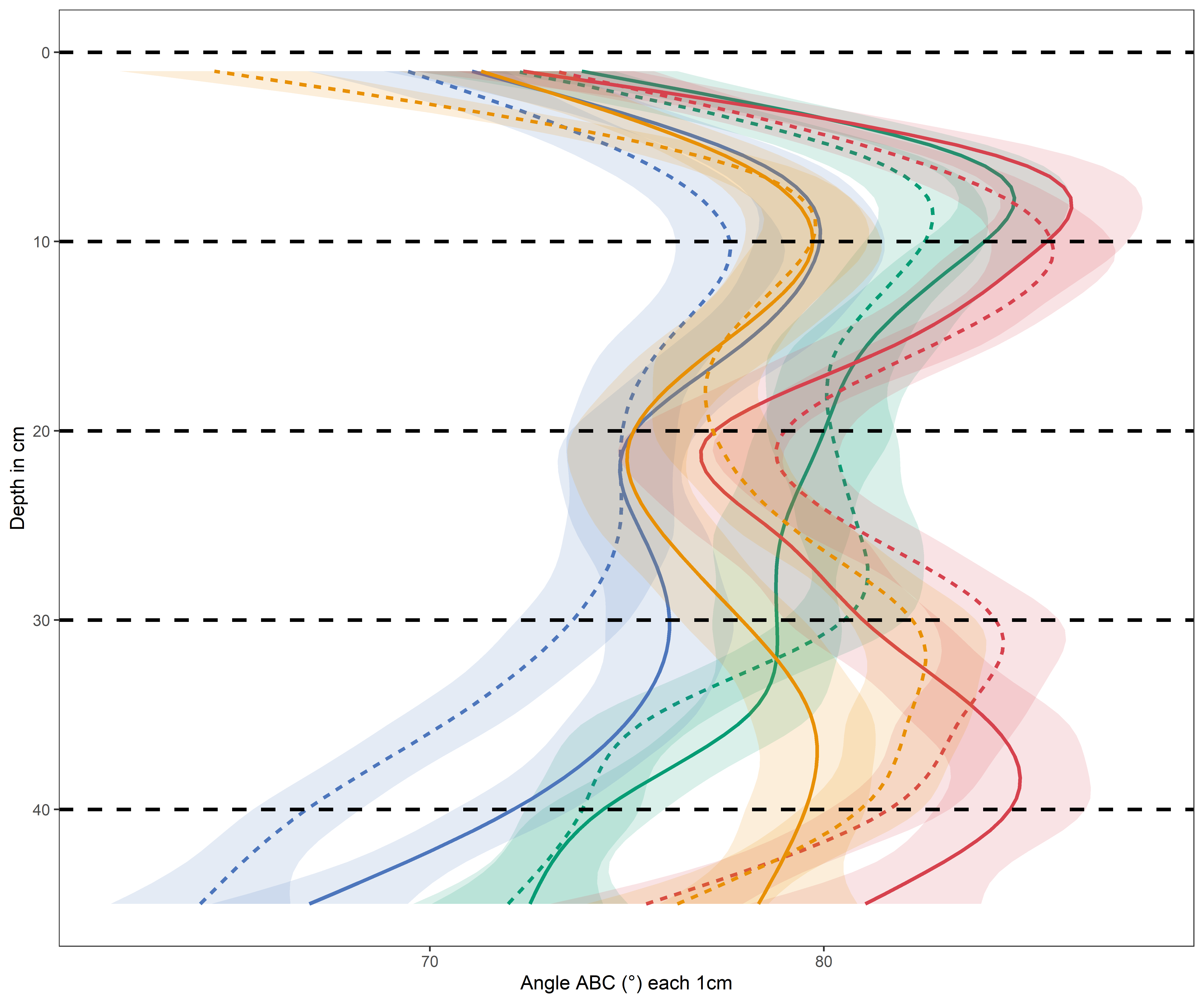
Is there a difference in angle depending on the depth in the rhizotube?
Code
a=1 ; b=10coo_root_angle_select$cut_break=cut(coo_root_angle_select$YB_calc_cm,breaks =c(seq(0,45+a,a)),labels=c(seq(0,45,a)),include.lowest =TRUE)p2=coo_root_angle_select %>%filter(!is.na(YB_calc_cm)) %>%filter(!is.na(cut_break)) %>%filter(YB_calc_cm<45) %>%filter(branching==1) %>%####### warningggplot(aes(x=as.numeric(as.character(cut_break)),y=Angle_ABC,colour=as.factor(condition))) +stat_summary(aes(group=as.factor(condition)),fun=mean,geom="line",size=1,alpha=0.85)+scale_x_continuous(limits =c(0,45))+xlab("Profondeur (cm")+ylab("Angle ABC (°)")+geom_vline(xintercept =seq(0,45,b) , linetype="dashed", color ="black", size=1)+ggtitle(paste("Mean eatch", a, "cm for line, for dashed line every",b, "cm",sep=" "))+scale_color_manual(values=climate_pallet)p2#with smooth function ?p3=coo_root_angle_select %>%filter(!is.na(YB_calc_cm)) %>%filter(!is.na(cut_break)) %>%filter(YB_calc_cm<45) %>%filter(branching==1) %>%####### warning#ggplot(aes(x=as.numeric(as.numeric(cut_break)*a),y=Angle_ABC,colour=as.factor(climat_condition),fill=as.factor(climat_condition)))+ggplot(aes(x=as.numeric(as.numeric(cut_break)*a),y=Angle_ABC,colour=as.factor(climat_condition),fill=as.factor(climat_condition),linetype=genotype))+#trop lourdgeom_smooth(alpha=.15)+#geom_point()+geom_vline(xintercept =seq(0,45,b) , linetype="dashed", color ="black", size=1)+#ggtitle(paste("Mean eatch", a, "cm for line, for dashed line every",b, "cm for branching 1",sep=" "))+scale_color_manual(values=climate_pallet)+scale_fill_manual(values=climate_pallet)+coord_flip() +scale_x_reverse()+labs(color="Treatment",fill="Treatment",linetype="Genotype")+theme_bw()+theme(panel.grid.major =element_blank(),panel.grid.minor =element_blank(),legend.position ="none")+xlab("Depth in cm")+ylab("Angle ABC (°) each 1cm")export_fig(p=p3,export_path = here::here("report/root_architecture/plot/angle_ABC_branching_1_by_profondeur_each_1cm.png"),export_height =20,export_width =24)
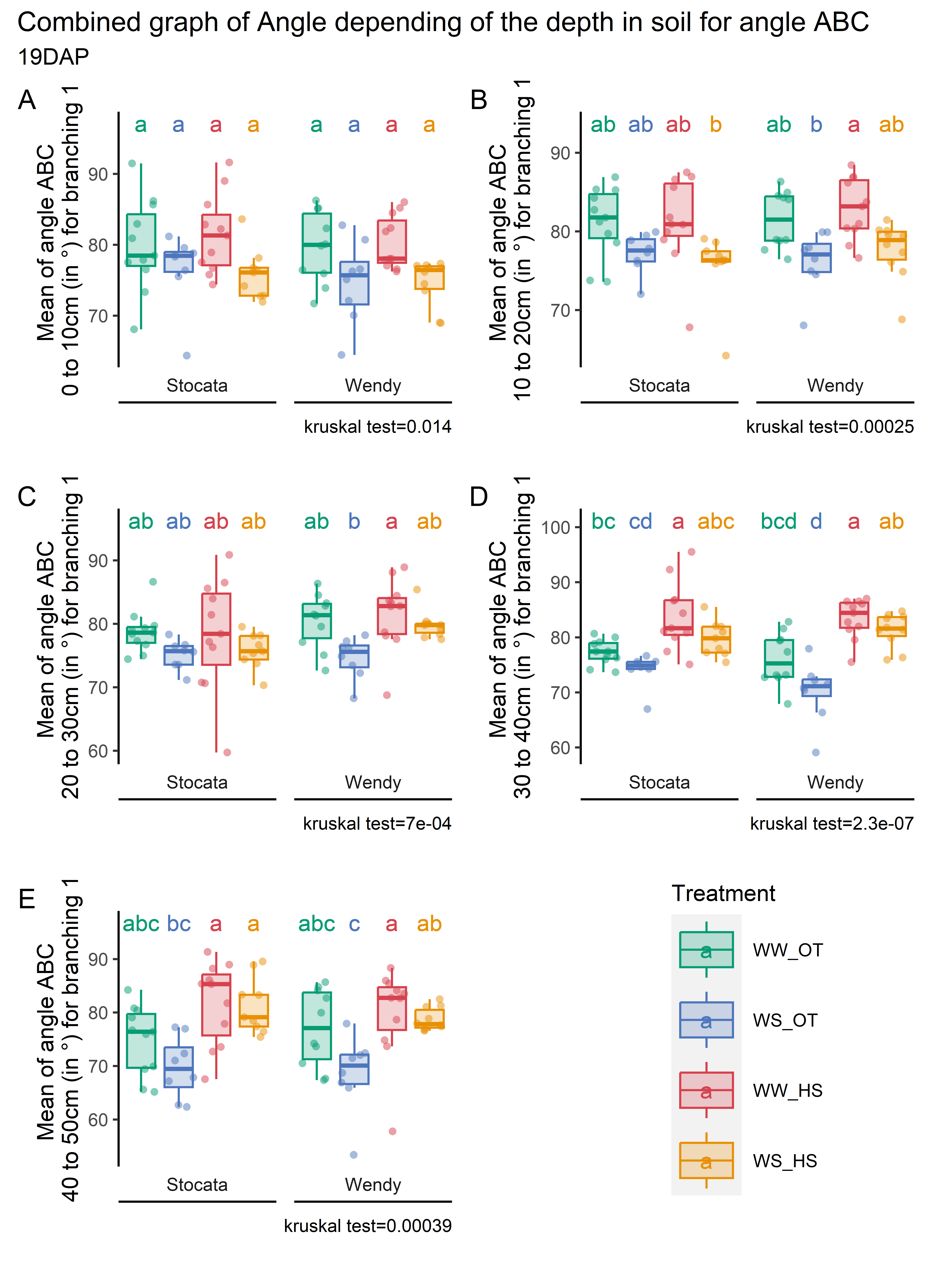
Verification of the hypothesis for a certain depth
Code
a=1 ; b=10coo_root_angle_select$cut_break=cut(coo_root_angle_select$YB_calc_cm,breaks =c(seq(0,60,10)),labels=c(seq(0,50,10)),include.lowest =TRUE)profondeurs=seq(0,40,10)plots <-lapply(1:length(profondeurs), function(i) { angle_for_plettre<-coo_root_angle_select %>%filter(branching==1) %>%#filter(plant_num!=1005) %>%filter(cut_break ==profondeurs[i]) %>% dplyr::group_by(condition,heat_condition,water_condition,genotype,plant_num) %>% dplyr::summarise(across(Angle_ABC:Angle_C2BD2, \(x) mean(x,na.rm=T)))%>%mutate(condition=factor(condition,levels=c("Wen_WW_OT","Wen_WW_HS","Wen_WS_OT","Wen_WS_HS","Sto_WW_OT","Sto_WW_HS","Sto_WS_OT","Sto_WS_HS")))FigX_stat=stat_analyse(data=angle_for_plettre %>%mutate(climat_condition=paste0(water_condition,"_",heat_condition)) %>%mutate(condition=factor(condition,levels=c("Sto_WW_OT","Stoc_WS_OT","Sto_WW_HS","Sto_WS_HS","Wen_WW_OT","Wen_WS_OT","Wen_WW_HS","Wen_WS_HS"))) %>%mutate(climat_condition=factor(climat_condition,levels=c("WW_OT","WS_OT","WW_HS","WS_HS"))) %>%drop_na(climat_condition,Angle_ABC),column_value ="Angle_ABC",category_variables =c("climat_condition"),grp_var ="genotype",show_plot = T,outlier_show = F, label_outlier ="plant_num",biologist_stats = T,Ylab_i =paste0("Mean of angle ABC \n",profondeurs[i]," to ",profondeurs[i]+10,"cm (°) for branching 1"),control_conditions =c("WW_OT"),strip_normale = F,hex_pallet = climate_pallet)px=FigX_stat[["plot"]] +theme(axis.title.x=element_blank(),axis.text.x=element_blank(),panel.grid.major =element_blank(),panel.grid.minor =element_blank(),legend.position ="right",plot.margin=unit(c(0.1,0.1,0.7,0.1), "cm"))#,plot.caption = element_text(vjust = 10))print(px)+labs(color="Treatment",fill="Treatment")})# Assembling graphicsfinal_plot <-wrap_plots(plots, ncol =2)+plot_layout(guides ="collect")+guide_area()+plot_annotation(tag_levels ='A',title="Combined graph of Angle depending of the depth in soil for angle ABC",subtitle="19DAP")png(here::here("report/root_architecture/plot/angle_ABC_depending_depth_19DAP_condition.png"), width =16, height =22, units ='cm', res =900)final_plotdev.off()
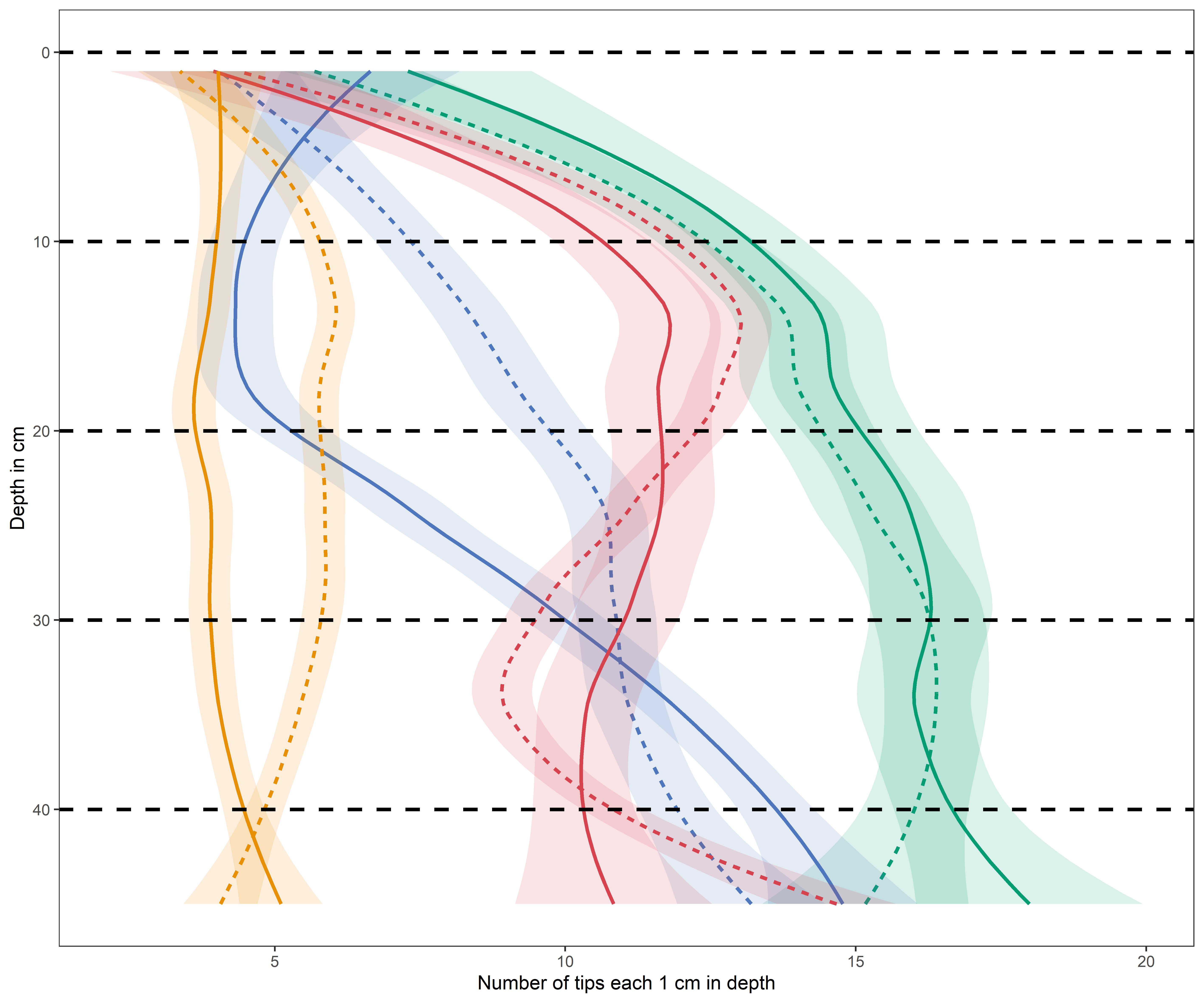
9.1.2 Number of tips
The number of root tips depending on the depth?
Code
a=1 ; b=10coo_root_tips_select$cut_break=cut(coo_root_tips_select$cm,breaks =c(seq(0,45+a,a)),labels=c(seq(0,45,a)),include.lowest =TRUE)p4=coo_root_tips_select %>%filter(!is.na(cm)) %>%filter(!is.na(cut_break)) %>%filter(cm<45) %>%ggplot(aes(x=as.numeric(as.character(cut_break)),y=X,colour=as.factor(condition))) +stat_summary(aes(group=as.factor(condition)),fun=length,geom="line",size=1,alpha=0.85)+scale_x_continuous(limits =c(0,45))+xlab("Profondeur (cm")+ylab("Number of root tips")+geom_vline(xintercept =seq(0,45,b) , linetype="dashed", color ="black", size=1)+ggtitle(paste("Mean eatch", a, "cm for line, for dashed line every (need verification because huge nuber of root tips",b, "cm",sep=" "))+scale_color_manual(values=climate_pallet)p4#export_png(p=p4,export_path = here::here(paste0("xp1_analyse/plot/root_architecture/by_profondeur/nb_tips_by_profondeur_cm.png")),export_height = 20,export_width = 24)#with smoothp5= coo_root_tips_select %>%filter(!is.na(cm)) %>%filter(!is.na(cut_break)) %>%filter(cm<45) %>% dplyr::group_by(climat_condition,heat_condition,water_condition,genotype,plant_num,cut_break) %>% dplyr::summarise(nb_tips =n()) %>%ggplot(aes(x=as.numeric(as.numeric(cut_break)*a),y=nb_tips,colour=climat_condition,fill=climat_condition,linetype=genotype))+geom_smooth(alpha=.15)+#geom_point()+geom_vline(xintercept =seq(0,45,b) , linetype="dashed", color ="black", size=1)+# ggtitle(paste("Mean eatch", a, "cm for line, for dashed line every",b, "cm using smooth",sep=" "))+scale_color_manual(values=climate_pallet)+ylab ("Number of tips each 1 cm in depth")+xlab("Depth in cm")+scale_fill_manual(values=climate_pallet)+coord_flip() +scale_x_reverse() +labs(color="Treatment",fill="Treatment",linetype="Genotype")+theme_bw()+theme(panel.grid.major =element_blank(),panel.grid.minor =element_blank(),legend.position ="none")#p3=p3+xlab("Depth in cm")+ylab("Mean angle ABC (°) each 1cm")# scale_y_continuous(trans = "reverse")p5export_fig(type ="png",p=p5,export_path = here::here(paste0("report/root_architecture/plot/nb_tips_by_profondeur_cm_smooth_mean1cm.png")),export_height =20,export_width =24)
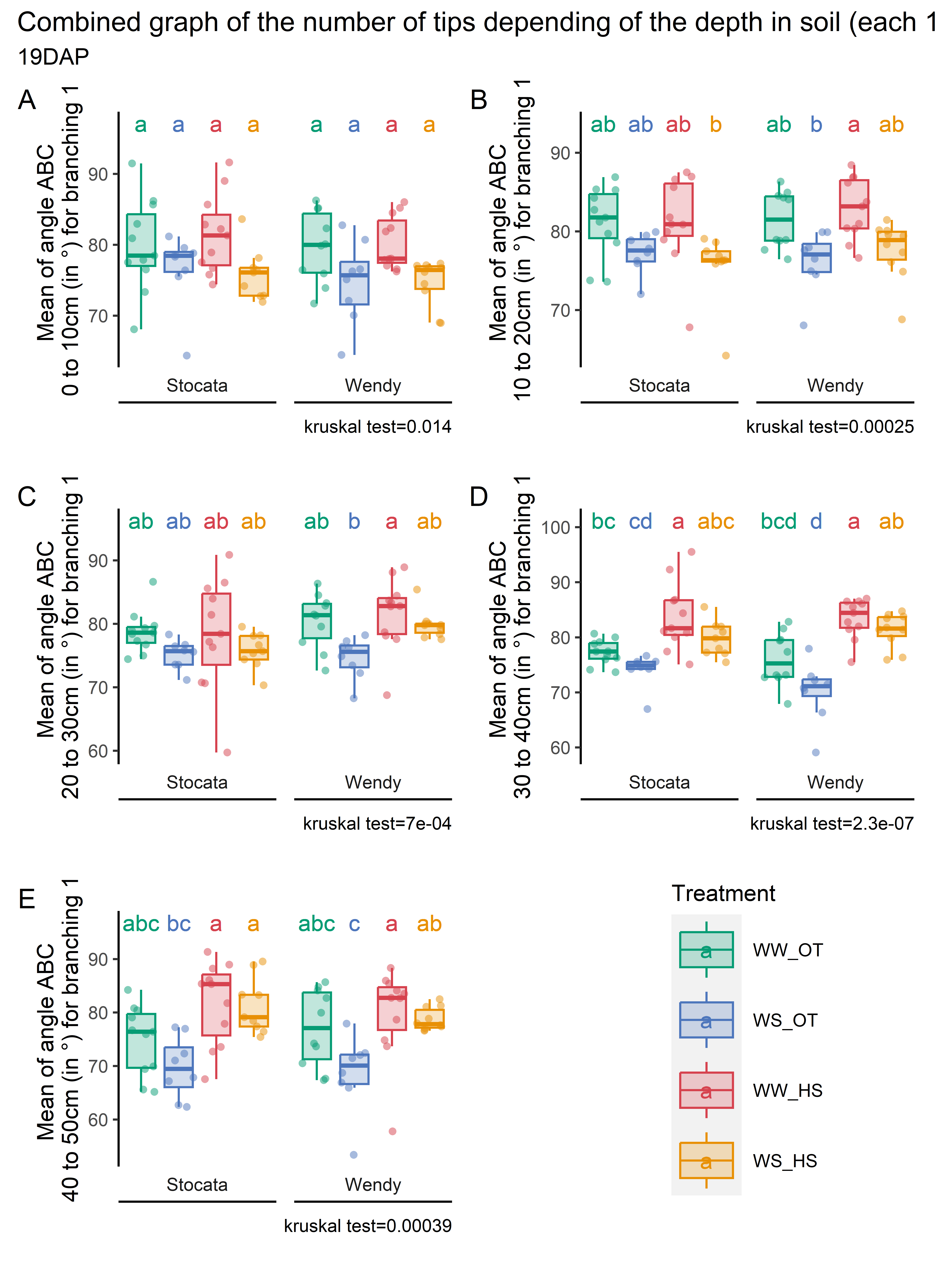
Verification of the hypothesis for a certain depth
Code
a=1 ; b=10coo_root_tips_select$cut_break=cut(coo_root_tips_select$cm,breaks =c(seq(0,60,10)),labels=c(seq(0,50,10)),include.lowest =TRUE)profondeurs=seq(0,40,10)tips_for_plettre <-lapply(1:length(profondeurs), function(i) { tips_for_plettre<-coo_root_tips_select %>%filter(plant_num!=1005) %>%filter(cut_break ==profondeurs[i]) %>% dplyr::group_by(condition,heat_condition,water_condition,genotype,plant_num) %>% dplyr::summarise(nb_tips =n()) %>%mutate(condition=factor(condition,levels=c("Wen_WW_OT","Wen_WW_HS","Wen_WS_OT","Wen_WS_HS","Sto_WW_OT","Sto_WW_HS","Sto_WS_OT","Sto_WS_HS")))#filter(branching==1) FigX_stat=stat_analyse(data=tips_for_plettre %>%mutate(climat_condition=paste0(water_condition,"_",heat_condition)) %>%mutate(condition=factor(condition,levels=c("Sto_WW_OT","Stoc_WS_OT","Sto_WW_HS","Sto_WS_HS","Wen_WW_OT","Wen_WS_OT","Wen_WW_HS","Wen_WS_HS"))) %>%mutate(climat_condition=factor(climat_condition,levels=c("WW_OT","WS_OT","WW_HS","WS_HS"))) %>%drop_na(climat_condition,nb_tips) %>%as.data.frame(),column_value ="nb_tips",category_variables =c("climat_condition"),grp_var ="genotype",show_plot = T,outlier_show = F, label_outlier ="plant_num",biologist_stats = T,Ylab_i =paste0("Number of tips in ",profondeurs[i]," to ",profondeurs[i] +10," cm"),control_conditions =c("WW_OT"),strip_normale = F,hex_pallet = climate_pallet ) px=FigX_stat[["plot"]] +theme(axis.title.x=element_blank(),axis.text.x=element_blank(),panel.grid.major =element_blank(),panel.grid.minor =element_blank(),legend.position ="right",plot.margin=unit(c(0.1,0.1,0.7,0.1), "cm"))#,plot.caption = element_text(vjust = 10))print(px)+labs(color="Treatment",fill="Treatment")})# Assembling graphicsfinal_plot <-wrap_plots(plots, ncol =2)+plot_layout(guides ="collect")+guide_area()+plot_annotation(tag_levels ='A',title="Combined graph of the number of tips depending of the depth in soil (each 10cm)",subtitle="19DAP")png(here::here("report/root_architecture/plot/nb_tips_depending_depth_19DAP_condition.png"), width =16, height =22, units ='cm', res =900)final_plotdev.off()
Again we have very good result depending of the depth