Import and compile raw watering and raw weighing data from the experiment
Warning, I have added the manual values realized on October 8, 2021.
Correction of the weights, According to the weight of the soil, the weight of the empty rhizotubes, the weight of the stakes and the mini-greenhouse
Import of substrate moisture data prior to the experiment and stake weights
Subtract or add the weight of each the Rhizotube, mini greenhouses or stake
Adding the weight of the mini greenhouses taking into account the date of presence of the mini greenhouses (given in the excel) First step, remove the inistial points from the rhizotube and add the fresh soil and dry soil data
Removed or added the weight corresponding to the minigreenhouse or the stake
Select the desired time interval (start and end of experiment) and delete the outliers
Add the information for each rhizotube (WS WW, HS, OT, genotype, date of harvest…)
Selection of rhizotubes that have two plants. Because if a plant does not germinate or has an abnormal phenotype it could induce errors for the evapotranspiration calculations
Note, that this must be based on fresh soil and dry soil.
Code
global_weight_select2 %>%mutate(time=format(as.POSIXct(global_weight_select2$resultdate_time), format ="%H:%M:%S")) %>%ggplot(aes(as.POSIXct(time, format="%H:%M:%S"), fill=resultdate)) +geom_density(alpha =0.5) +#also play with adjust such as adjust = 0.5scale_x_datetime(breaks =date_breaks("2 hours"), labels=date_format("%H:%M")) +labs(x="Houre in the day")
3.2 Water in the rhizotube
Take the desired time interval and the least defective watering stations
Code
global_weight_select3<-global_weight_select2%>%filter(as.Date(resultdate)>as.Date("2021-09-22")) %>%filter(weightafter>15000) %>%filter(usedstationid %in%c("26","36")) %>%filter(type %in%c("weighing", "watering")) %>%mutate(day=as.POSIXct(resultdate_time)-as.POSIXct("2021-09-23 00:00:00"))write.csv(global_weight_select3, "data/water/weighing_watering_output/global_weight_select3.csv")p1<-ggplot(global_weight_select3, aes(x=day, y=water_in_rt, colour=paste0(condition,"_",usedstationid), group=c(paste0(condition,"_",usedstationid)))) +geom_point(size=0.7,alpha=.4)+geom_smooth()+labs(x="Date of watering or weighing",y="Water in Rhizotube (ml)",color="condition \n+usedstationid")+guides(colour =guide_legend(nrow =3, byrow = T))+scale_x_continuous(breaks =round(seq(min(as.integer(global_weight_select3$day)), as.integer(max(global_weight_select3$day)), by =2),1))+theme_minimal()+theme(legend.position="bottom")error_balance_begin_XP=0.01p_soil_water_content<-ggplot( global_weight_select3 %>%filter(recolte==2) %>%filter(day>2) %>%mutate(climat_condition=paste0(water_condition,"_",heat_condition)) %>%mutate(humidity=ifelse(climat_condition=="WS_HS",humidity+error_balance_begin_XP,humidity)) %>%mutate(condition=factor(condition,levels=c("Sto_WW_OT","Sto_WW_HS","Sto_WS_OT","Sto_WS_HS","Wen_WW_OT","Wen_WW_HS","Wen_WS_OT","Wen_WS_HS"))) %>%mutate(climat_condition=factor(climat_condition,levels=c("WW_OT","WS_OT","WW_HS","WS_HS"))) , aes(x=day-1, y=humidity, col=climat_condition,fill=climat_condition,linetype=genotype)) +geom_rect(xmin =5, xmax =20, ymin =-Inf, ymax =0.11, fill ="#c9d5ea", alpha =0.5,col="gray") +geom_rect(xmin =5, xmax =10, ymin =-Inf, ymax =Inf, fill ="lightgray", alpha =0.02,col="gray") +geom_rect(xmin =15, xmax =20, ymin =-Inf, ymax =Inf, fill ="lightgray", alpha =0.02,col="gray") +geom_point(size=0.7,alpha=.4)+geom_smooth()+labs(x="Number of days after transplantation",y="Soil water content (%)",color="Treatment",fill="Treatment",linetype="Genotype")+guides(colour =guide_legend(nrow =3, byrow = T))+# scale_x_continuous(breaks = round(seq(min(as.integer(global_weight_select3$day)), as.integer(max(global_weight_select3$day)), by = 5),1))+#scale_x_datetime(date_breaks= "2 days", date_minor_breaks = "12 hour")+#scale_y_continuous(breaks=1)scale_color_manual(values=climate_pallet)+scale_fill_manual(values=climate_pallet)+theme(legend.position="right")+ my_theme# ggsave(here::here("report/water/plot/Water_in_RT.svg"), # p1, width = 20,height = 16, units = "cm")ggsave(here::here("report/water/plot/Water_in_RT.png"), p1, width =20, height =16, units ="cm", dpi =600)# ggsave(here::here("report/water/plot/soil_water_content.svg"), # p_soil_water_content, width = 20,height = 16, units = "cm")ggsave(here::here("report/water/plot/soil_water_content.png"), p_soil_water_content, width =20, height =16, units ="cm", dpi =600)
Figure 3.1
Find the date of the next measurement for the same rizotube. Attention the last measurement is deleted.
3.3 Evapotranspiration
3.3.1 Kinetics
Caution
Be careful, this step takes a lot of time This step also adds a night day column and a night morning and afternoon column. This part also measures the time between two weighings
Code
# /!\ take time 5 min at leastcat_col("Caution: you have to wait a long time here", "red")global_weight_select3=read.csv("data/water/weighing_watering_output/global_weight_select3.csv")[-1]global_weight_select3$next_weight=NAlevels_factor_plant_id=levels(as.factor(global_weight_select3$plant_id))pb =txtProgressBar(min =0, max =length(levels_factor_plant_id), initial =0,style=3)#progresse bar for (i in levels_factor_plant_id){setTxtProgressBar(pb,match(i,levels_factor_plant_id)) #progresse bar data_watering_select_x=global_weight_select3 %>%filter(plant_id==i) %>%arrange(resultdate_time) levels_factor_resultdate_time=data_watering_select_x$resultdate_timefor (j in1:length(levels_factor_resultdate_time)){for (k in1:length(global_weight_select3$studyname)){if(as.character(global_weight_select3$plant_id[k])==i){# print(data_watering_select$plantid[k]) if(global_weight_select3$resultdate_time[k]==levels_factor_resultdate_time[j]){ global_weight_select3$next_weight[k]=as.character(levels_factor_resultdate_time[j+1])#print(paste(i,levels_factor_resultdate_time[j],levels_factor_resultdate_time[j+1], sep="_")) } } } }}df_evapotranspi=global_weight_select3 %>%drop_na(next_weight)df_evapotranspi$water_after=NApb =txtProgressBar(min =0, max =length(df_evapotranspi$studyname), initial =0,style=3)#progresse bar for (i in1:length(df_evapotranspi$studyname)){for (j in1:length(global_weight_select3$studyname)){if(df_evapotranspi$plant_id[i]==global_weight_select3$plant_id[j]){if (df_evapotranspi$next_weight[i]==global_weight_select3$resultdate_time[j]){ df_evapotranspi$water_after[i]=global_weight_select3$water_in_rt[j] } } }setTxtProgressBar(pb,i) #progresse bar}df_evapotranspi$evapotranspiration=df_evapotranspi$water_in_rt-df_evapotranspi$water_after+df_evapotranspi$deliveredquantity#diff time enter the two weightdf_evapotranspi$diff_resultdate_time=as.POSIXct(df_evapotranspi$next_weight)-as.POSIXct(df_evapotranspi$resultdate_time)#transforme date time of next_weight in juste time for separate by morning afternoone nightdf_evapotranspi$next_weight_time=format(strftime(df_evapotranspi$next_weight, format ="%H:%M:%S"))df_evapotranspi$night_day=NApb =txtProgressBar(min =0, max =length(df_evapotranspi$studyname), initial =0,style=3)#progresse bar for (i inseq_along(df_evapotranspi$studyname)){if (format(strftime(df_evapotranspi$next_weight[i], format ="%H:%M:%S"))<format(strftime("2021-10-01 09:18:00", format ="%H:%M:%S"))){if (format(strftime(df_evapotranspi$resultdate_time[i], format ="%H:%M:%S"))>format(strftime("2021-10-01 17:00:00", format ="%H:%M:%S"))){# print(paste(data_watering_select_transpiration_select$time[i],data_watering_select_transpiration_select$next_weight_time[i],sep="_")) df_evapotranspi$night_day[i]="night" }else{ df_evapotranspi$night_day[i]="day" } }else{ df_evapotranspi$night_day[i]="day" }setTxtProgressBar(pb,i) #progresse bar }df_evapotranspi$morning_afternoon="night"pb =txtProgressBar(min =0, max =length(df_evapotranspi$studyname), initial =0,style=3) #progresse bar for (i inseq_along(df_evapotranspi$studyname)){if(df_evapotranspi$night_day[i]=="day"){if(format(strftime(df_evapotranspi$resultdate_time[i], format ="%H:%M:%S"))<format(strftime("2021-10-01 11:00:00", format ="%H:%M:%S"))){ df_evapotranspi$morning_afternoon[i]="morning" }else(df_evapotranspi$morning_afternoon[i]="afternoon") }setTxtProgressBar(pb,i) #progresse bar }write.csv(df_evapotranspi,here::here("data/water/weighing_watering_output/df_evapotranspi.csv"))
Plot exemple for RT1067
Code
df_evapotranspi=read.csv(here::here("data/water/weighing_watering_output/df_evapotranspi.csv"))[-1]df_evapotranspi$resultdate_time=as.POSIXct(df_evapotranspi$resultdate_time)plot_x=df_evapotranspi %>%filter(plant_id=="1069")%>%ggplot(aes(x=resultdate_time, y=evapotranspiration/2, colour=paste0(condition,"_",usedstationid), group=c(paste0(condition,"_",usedstationid)))) +geom_smooth(se=F)+geom_point()+scale_x_datetime(breaks=("1 day"), minor_breaks=("1 hour"),labels =date_format("%b-%d %H:%M:%S"))+labs(x="Date and time", y="Evapotranspiration for one plante of one \n rhizotube (ml) between two watering or weighing",color="condition \n+usedstationid")+theme_minimal()+theme(axis.text.x =element_text(angle =90, hjust =1)) +theme(legend.position="bottom")ggsave(here::here("report/water/plot/evapotranspiration_1069.svg"), plot_x, width =20,height =16, units ="cm")
plot_x=sum_by_date %>%mutate(Group.1=factor(Group.1,levels=c("Sto_WW_OT","Sto_WW_HS","Sto_WS_OT","Sto_WS_HS","Wen_WW_OT","Wen_WW_HS","Wen_WS_OT","Wen_WS_HS"))) %>%ggplot(aes(x=as.factor(Group.3),y=x/2,fill=Group.2))+geom_boxplot(outlier.alpha =0)+#facet_grid(Group.5~.)+#geom_point(position=position_jitterdodge(),alpha=0.3)+theme(axis.text.x =element_text(angle =90, vjust =0.5, hjust=1))+scale_fill_manual(values=manu_palett)+labs(x="Date", y="Evapotranspiration for one plante of one rhizotube (ml) during on day")+theme(legend.position="bottom")ggsave(here::here("report/water/plot/evapotranspiration_each_plant.svg"), plot_x, width =20,height =16, units ="cm")
Error detection
Code
plot_x<- df_evapotranspi %>%mutate(condition=factor(condition,levels=c("Sto_WW_OT","Sto_WW_HS","Sto_WS_OT","Sto_WS_HS","Wen_WW_OT","Wen_WW_HS","Wen_WS_OT","Wen_WS_HS"))) %>%ggplot(aes(x=as.POSIXct(format(as.POSIXct(resultdate_time),format ="%H:%M:%S"),format ="%H:%M:%S"),y=evapotranspiration/2,col=condition))+geom_point()+facet_wrap(~resultdate)+scale_color_manual(values=manu_palett)+theme(axis.text.x =element_text(angle =90, vjust =0.5, hjust=1))+labs(y="Evapotranspiration between two weighings (ml) for one plant", x="Date time")+theme(legend.position="bottom")ggsave(here::here("report/water/plot/find_error_evapo.svg"), plot_x, width =20,height =18, units ="cm")
Sometimes have less than three waterings per day and at different times or more than 3. This can lead to calculation errors later on the script.
Code
plot_x<- df_evapotranspi %>%mutate(condition=factor(condition,levels=c("Sto_WW_OT","Sto_WW_HS","Sto_WS_OT","Sto_WS_HS","Wen_WW_OT","Wen_WW_HS","Wen_WS_OT","Wen_WS_HS"))) %>%ggplot(aes(x=as.POSIXct(format(as.POSIXct(resultdate_time),format ="%H:%M:%S"),format ="%H:%M:%S"),y=diff_resultdate_time/60,col=condition))+labs(y="Time (hours) between two weighing measurements for each rhizotube", x="Date and time")+geom_point()+facet_wrap(~resultdate)+scale_color_manual(values=manu_palett)+theme(axis.text.x =element_text(angle =90, vjust =0.5, hjust=1))+theme(legend.position="bottom")ggsave(here::here("report/water/plot/find_error_evapo_time_between.svg"), plot_x, width =20,height =18, units ="cm")
Why do I have the RT 1035 which has such a huge value between two waterings? Because there are missing values for the 1035 between the 27th at 7:45 and the 29th at 12:06. On the 27th the measurements of 14:27, 18:05 and 20:30 are missing. On the 28th the data of 6:06, 12:05 and 18:05 and on the 29th the data of 6:06.
Division of the evapotranspiration by the time between two weighing measurements. That is, divide by the weight after watering minus the weight before watering.
Code
#if i divide one by onedf_evapotranspi$div=df_evapotranspi$evapotranspiration/(as.numeric(df_evapotranspi$diff_resultdate_time)/60)plot_x<- df_evapotranspi %>%mutate(condition=factor(condition,levels=c("Sto_WW_OT","Sto_WW_HS","Sto_WS_OT","Sto_WS_HS","Wen_WW_OT","Wen_WW_HS","Wen_WS_OT","Wen_WS_HS"))) %>%filter(div>-1) %>%ggplot(aes(x=as.POSIXct(format(as.POSIXct(resultdate_time),format ="%H:%M:%S"),format ="%H:%M:%S"),y=div/2,col=condition))+geom_point(size=1.2, alpha=.5)+labs(y=expression(paste("Evapotranspiration of a plant per rhizotube (ml.",hour^{-1},")")), x="Date and time")+facet_wrap(~resultdate)+scale_color_manual(values=manu_palett)+theme(axis.text.x =element_text(angle =90, vjust =0.5, hjust=1))+theme(legend.position="bottom")ggsave(here::here("report/water/plot/evapo_by_plant_per_RT.svg"), plot_x, width =22,height =18, units ="cm")
Then I remove some aberrant data or that could bother me for the calculations. I remove the values of 2021-09-24 because the last weighing was done at 15h. I also remove the time between two weighing more than 16h30 and finally I remove the results of rhizotube 3 (aberrant results).
If I separate the evaporation between day and night. If I separate the evapotranspiration between day and night. One can see logically that evapotranspiration is much lower at night than during the day. During the day and in the course of the experiment, there is an increasing increase in evapotranspiration for plants in well-watered conditions. During the day, and during the first heat wave (from day X to day X), evapotranspiration increases for both genotypes, and then returns to a state close to the one observed in plants in optimal temperature conditions. During the second heat wave (from day X to day X), during the day and in well-watered conditions, there could be have a difference between the two genotypes. Wendy could be have a higher evapotranspiration in this condition. Can this be explained by their different aerial and root architecture (for the same biomass)? Towards the end we can see the re-watering of the plants in stressed condition.
Figure 3.2
If we look at the differences between conditions for each period of the day (morning, afternoon, evening) but not in ml.hours but in cumulative. There does not seem to be any major difference in evapotranspiration between these three periods.
Since we have chosen to make correlations between variables measured by plant and the efficiencies of water, element, radiation … we have chosen to make averages on the first harvest and to make calculations with these averages (H1) vs harvest 2 (HS).
Code
df_use_for_WUE=merge(read.csv(here::here("data/water/weighing_watering_output/df_evapo3.csv")) %>%drop_na(evapotranspiration)%>%drop_na(sum_biomass),as.data.frame(read.csv(here::here("data/water/weighing_watering_output/df_evapo3.csv")) %>%group_by(plant_id, condition, recolte) %>% dplyr::summarise(.groups ='drop',sum_total_evapotranspiration=sum(evapotranspiration)) %>%drop_na(sum_total_evapotranspiration)) %>% dplyr::select(plant_id,sum_total_evapotranspiration ) %>%drop_na(sum_total_evapotranspiration),all=T, by="plant_id") %>%group_by(recolte,condition)%>% dplyr::summarise(mean_sum_biomass =mean(sum_biomass),mean_sum_total_evapotranspiration=mean(sum_total_evapotranspiration),.groups ='drop') %>%#.groups = 'drop' for delet warning messagedrop_na(mean_sum_biomass) %>%as.data.frame() %>%mutate(mean_sum_biomass=mean_sum_biomass*1000) %>%mutate(mean_sum_total_evapotranspiration=mean_sum_total_evapotranspiration/2)kbl(df_use_for_WUE, caption ="Resume of the data use for Water Use Efficiency (WUE) for eatch condition",col.names=c("Harvest","Condition", "Average total weight (mg)", "Average total evapotranspiration (ml)"),digits =1) %>%kable_paper(full_width = F) %>%#column_spec(3, color = "white",background = spec_color(WUE$mean_sum_biomass, end = 0.7))%>%column_spec(4, color ="white",background =spec_color(df_use_for_WUE$mean_sum_biomass, end =0.7))
Resume of the data use for Water Use Efficiency (WUE) for eatch condition
Harvest
Condition
Average total weight (mg)
Average total evapotranspiration (ml)
1
Sto_WW_OT
89.3
70.2
1
Wen_WW_OT
88.0
70.3
2
Sto_WS_HS
287.8
498.7
2
Sto_WS_OT
471.0
446.1
2
Sto_WW_HS
1050.2
1750.4
2
Sto_WW_OT
1195.4
1569.4
2
Wen_WS_HS
360.1
484.3
2
Wen_WS_OT
527.9
449.2
2
Wen_WW_HS
1281.2
1863.1
2
Wen_WW_OT
1260.7
1608.1
3.4.1 WUE with mean in H1 and H2
Water Use Efficiency, Thesis Couchoud (p69): Stomata closure may not be complete, transpiration is then more reduced than the net assimilation of atmospheric CO2 by photosynthesis. An increase in water use efficiency (WUE) is then observed (Maury et al., 2011). This change in WUE in response to water stress has been reported in multiple studies and high WUE is commonly associated with better tolerance to water stress (Chaves et al., 2003, 2009; Siopongco et al., 2006; Xu et al., 2010; Anjum et al., 2011; Erice et al., 2011).
Water Use Efficiency (WUE) between date t1 and t2 was calculated as the ratio of the plant biomass (BM) accumulated over the amount of water evapotranspirated by the plant during this period (QH2O) and is expressed in g. gH2O-1:
Code
# Process to calculWUE2mean=df_use_for_WUEWUE2mean$result_WUE=NAfor (i in1:nrow(WUE2mean)){for (j in1:nrow(WUE2mean)){if (WUE2mean$recolte[i]==1){ WUE2mean$result_WUE[i]=NA }elseif (WUE2mean$recolte[i]==2&& WUE2mean$recolte[j]==1){if(str_sub(WUE2mean$condition[i], 1, 3)==str_sub(WUE2mean$condition[j], 1, 3)){ WUE2mean$result_WUE[i]=(WUE2mean$mean_sum_biomass[i]/1000-WUE2mean$mean_sum_biomass[j]/1000)/(((WUE2mean$mean_sum_total_evapotranspiration[i]/1000))-((WUE2mean$mean_sum_total_evapotranspiration[j]/1000))) } } }}write.csv(WUE2mean,here::here("data/water/weighing_watering_output/WUE_with_mean_h1_and_mean_h2.csv"))
Code
# show tableread.csv(here::here("data/water/weighing_watering_output/WUE_with_mean_h1_and_mean_h2.csv")) %>%dplyr::select(recolte,condition,mean_sum_biomass, mean_sum_total_evapotranspiration, result_WUE) %>%mutate(mean_sum_biomass=mean_sum_biomass/1000,mean_sum_total_evapotranspiration=(mean_sum_total_evapotranspiration/1000),result_WUE=result_WUE) %>%kbl(caption ="WUE for eatch condition. Only mean using",col.names=c("Harvest","Condition", "Dry weight total (g)", "Sum of the evapotranspiration (L)", "WUE (g. L H20-1)"), digits =2) %>%kable_paper(full_width = F) %>%column_spec(5, color ="white",background =spec_color(read.csv(here::here("data/water/weighing_watering_output/WUE_with_mean_h1_and_mean_h2.csv")) %>%pull(result_WUE), end =0.7))
WUE for eatch condition. Only mean using
Harvest
Condition
Dry weight total (g)
Sum of the evapotranspiration (L)
WUE (g. L H20-1)
1
Sto_WW_OT
0.09
0.07
NA
1
Wen_WW_OT
0.09
0.07
NA
2
Sto_WS_HS
0.29
0.50
0.46
2
Sto_WS_OT
0.47
0.45
1.02
2
Sto_WW_HS
1.05
1.75
0.57
2
Sto_WW_OT
1.20
1.57
0.74
2
Wen_WS_HS
0.36
0.48
0.66
2
Wen_WS_OT
0.53
0.45
1.16
2
Wen_WW_HS
1.28
1.86
0.67
2
Wen_WW_OT
1.26
1.61
0.76
3.4.2 WUE and sRWU (H1 mean )
Code
# Data importation and preparation for H1 and H2df_H1_mean<-merge(sum_evapo_end %>%filter(recolte==1),read.csv2(here::here("data/physio/global_physio.csv")) %>% dplyr::select(plant_id, weight_root,sum_biomass, plant_num,genotype,date_recolte,recolte) %>%filter(recolte==1) %>% dplyr::select(-recolte),by="plant_id", all=T) %>%drop_na(weight_root,sum_total_evapotranspiration) %>%mutate(sum_total_evapotranspiration=sum_total_evapotranspiration/1000/2) %>% dplyr::group_by(condition, genotype,recolte,date_recolte) %>% dplyr::summarise(across(sum_total_evapotranspiration:sum_biomass, ~mean(.x, na.rm =TRUE))) %>% dplyr::rename_all(~paste0(., "_H1")) %>% dplyr::rename(genotype=genotype_H1)df_H2<-merge(sum_evapo_end %>%filter(recolte==2),read.csv2(here::here("data/physio/global_physio.csv")) %>% dplyr::select(plant_id, weight_root,sum_biomass, plant_num,genotype,date_recolte,recolte) %>%filter(recolte==2) %>% dplyr::select(-recolte),by="plant_id", all=T) %>%drop_na(weight_root,sum_total_evapotranspiration) %>%mutate(sum_total_evapotranspiration=sum_total_evapotranspiration/1000/2) %>% dplyr::rename_all(~paste0(., "_H2")) %>% dplyr::rename(genotype=genotype_H2)# Process WUE and sRWUWUE_sRWU_1mean=full_join(df_H2, df_H1_mean, by="genotype",relationship ="many-to-many") %>%mutate(WUE=(sum_biomass_H2 -sum_biomass_H1)/(sum_total_evapotranspiration_H2 -sum_total_evapotranspiration_H1)) %>%mutate(sRWU=(sum_total_evapotranspiration_H2-sum_total_evapotranspiration_H1)/ (( (as.numeric(as.Date(date_recolte_H2)-as.Date(date_recolte_H1))) * ((weight_root_H2+weight_root_H1)/2) ))) %>% dplyr::rename(condition=condition_H2) %>%mutate(water_condition=str_sub(condition, 5, 6)) %>%mutate(heat_condition=str_sub(condition, 8, 9)) %>%mutate(climat_condition=paste0(water_condition, "_", heat_condition)) %>%mutate(condition=factor(condition,levels=c("Sto_WW_OT","Sto_WS_OT","Sto_WW_HS","Sto_WS_HS","Wen_WW_OT","Wen_WS_OT","Wen_WW_HS","Wen_WS_HS"))) %>%mutate(climat_condition=factor(climat_condition,levels=c("WW_OT","WS_OT","WW_HS","WS_HS")))# export resultswrite.csv(WUE_sRWU_1mean,here::here(paste(sep="_","data/water/weighing_watering_output/WUE_sRWU_1mean.csv")))# Show resultspWUE=stat_analyse(data =WUE_sRWU_1mean,column_value ="WUE",category_variables =c("climat_condition"),grp_var ="genotype",control_conditions =c("WW_OT"),biologist_stats = T,strip_normale = F,outlier_show = F,label_outlier ="plant_num_H2",show_plot = T,hex_pallet = climate_pallet,Ylab_i =paste0("Water Use Efficiency (g/L)") )pWUE<-pWUE[["plot"]]+labs(color="Treatment",fill="Treatment")+theme(axis.title.x=element_blank(),axis.text.x=element_blank(),panel.grid.major =element_blank(),panel.grid.minor =element_blank(),axis.ticks.x =element_blank() )+labs(subtitle ="WUE with one mean")# Show resultspsRWU=stat_analyse(data =WUE_sRWU_1mean,column_value ="sRWU",category_variables =c("climat_condition"),grp_var ="genotype",control_conditions =c("WW_OT"),biologist_stats = T,strip_normale = F,outlier_show = F,label_outlier ="plant_num_H2",show_plot = T,hex_pallet = climate_pallet,Ylab_i =paste0("specific Root Water Uptake (gH2O[gBMroot day-1]-1)") )psRWU<-psRWU[["plot"]]+labs(color="Treatment",fill="Treatment")+theme(axis.title.x=element_blank(),axis.text.x=element_blank(),panel.grid.major =element_blank(),panel.grid.minor =element_blank(),axis.ticks.x =element_blank() )+labs(subtitle ="sRWU with one mean")combined_plot<-(pWUE+psRWU) +plot_layout(guides ='collect')# export figurepng(here::here(paste0("report/water/plot/WUE_sRWU_1mean.png")), width =18, height =10, units ='cm', res =900)combined_plotdev.off()
Code
# show tableread.csv(here::here("data/water/weighing_watering_output/WUE_sRWU_1mean.csv")) %>%dplyr::select(condition, WUE,sRWU) %>% dplyr::group_by(condition) %>% dplyr::summarise(across(WUE:sRWU, mean, na.rm =TRUE)) %>%kbl(caption ="WUE and sRWU for eatch condition. Mean only for H1", col.names=c("Condition", "WUE (g. L H20-1)","sRWU(gH2O[gBMroot day-1]-1)"), digits =2) %>%kable_paper(full_width = F) %>%column_spec(2, color ="white",background =spec_color(read.csv(here::here("data/water/weighing_watering_output/WUE_sRWU_1mean.csv")) %>%dplyr::group_by(condition) %>% dplyr::summarise(across(WUE:sRWU, mean, na.rm =TRUE)) %>%pull(WUE), end =0.7)) %>%column_spec(3, color ="white",background =spec_color(read.csv(here::here("data/water/weighing_watering_output/WUE_sRWU_1mean.csv")) %>%dplyr::group_by(condition) %>%dplyr::summarise(across(WUE:sRWU, mean, na.rm =TRUE)) %>%pull(sRWU), end =0.7))
WUE and sRWU for eatch condition. Mean only for H1
Condition
WUE (g. L H20-1)
sRWU(gH2O[gBMroot day-1]-1)
Sto_WS_HS
0.47
0.66
Sto_WS_OT
1.03
0.35
Sto_WW_HS
0.57
1.03
Sto_WW_OT
0.74
0.74
Wen_WS_HS
0.67
0.54
Wen_WS_OT
1.18
0.32
Wen_WW_HS
0.65
0.98
Wen_WW_OT
0.77
0.77
3.4.3 WUE and sRWU (Drawing with discount )
Now according to Marion, I have to do random draw for statistical analysis see script used for nodosity in my first paper. I have a repetition of the draw of 100 for eatch condition according to Denis Vile. The problem is that I have lots of data warning of different df. Already only one measurement for root weight. So I have to halve the evapotranspiration because I don’t know which RT plant it is.
Code
# Data generationdf_WUE_sRWU_bootstrap=merge(sum_evapo_end,read.csv2(here::here("data/physio/global_physio.csv")) %>% dplyr::select(plant_id, weight_root,sum_biomass, plant_num,genotype,date_recolte),by="plant_id", all=T ) %>%drop_na(weight_root,sum_total_evapotranspiration) %>%mutate(sum_total_evapotranspiration=sum_total_evapotranspiration/1000/2)# Process to bootstraplist_condition<-levels(as.factor(df_WUE_sRWU_bootstrap$condition))### parameter rep=100set.seed(1)df_bootstrap=data.frame()#For eatch condition of the harvest 2for (i in1:rep){for (cond_x in list_condition){ df_x=df_WUE_sRWU_bootstrap %>%filter(recolte=="2") %>%filter(condition==cond_x) df_x_taking=df_x %>%filter(plant_num==sample(df_x$plant_num,1,replace=T)) if(str_sub(df_x_taking$condition, 1, 3)=="Sto"){ df_y=df_wue %>%filter(recolte=="1") %>%filter(genotype=="Stocata") }else { df_y=df_wue %>%filter(recolte=="1") %>%filter(genotype=="Wendy") } df_y_taking=df_y %>%filter(plant_num==sample(df_y$plant_num,1,replace=T)) colnames(df_x_taking)=c("plant_id_rec_2","condition","recolte_2","sum_evapo_transpi_2","weight_root_2","weight_tot_2","plant_num_2","genotype_2","date_recolte_2")colnames(df_y_taking)=c("plant_id_rec_1","condition1","recolte_1","sum_evapo_transpi_1","weight_root_1","weight_tot_1","plant_num_1","genotype_1","date_recolte_1") df_bind=cbind(df_y_taking,df_x_taking) df_bind$rep=i df_bind$simulation=paste0(i,"_",cond_x) df_bind$WUE=(df_bind$weight_tot_2-df_bind$weight_tot_1)/(df_bind$sum_evapo_transpi_2-df_bind$sum_evapo_transpi_1) df_bind$sRWU=(df_bind$sum_evapo_transpi_2-df_bind$sum_evapo_transpi_1)/ (( (as.numeric(as.Date(df_bind$date_recolte_2)-as.Date(df_bind$date_recolte_1))) * ((df_bind$weight_root_2+df_bind$weight_root_1)/2) ))#print(str_sub(df_x_taking$condition, 1, 3)) df_bootstrap=rbind(df_bootstrap,df_bind) } fit <-aov(WUE ~ condition, df_compile)# analyse de varianceprint(summary(fit)[[1]][["Pr(>F)"]][1]) ; }# Obviously the more loops i make the stronger i am !!! df_bootstrap=df_bootstrap %>%mutate(water_condition=str_sub(condition, 5, 6)) %>%mutate(heat_condition=str_sub(condition, 8, 9)) %>%mutate(climat_condition=paste0(water_condition, "_", heat_condition)) %>%mutate(condition=factor(condition,levels=c("Sto_WW_OT","Sto_WS_OT","Sto_WW_HS","Sto_WS_HS","Wen_WW_OT","Wen_WS_OT","Wen_WW_HS","Wen_WS_HS"))) %>%mutate(climat_condition=factor(climat_condition,levels=c("WW_OT","WS_OT","WW_HS","WS_HS"))) %>% dplyr::rename(genotype=genotype_2)# export resultswrite.csv(df_bootstrap,here::here(paste(sep="_","data/water/weighing_watering_output/WUE_sRWU_Bootstrap.csv")))# Show resultspWUE=stat_analyse(data =df_bootstrap,column_value ="WUE",category_variables =c("climat_condition"),grp_var ="genotype",control_conditions =c("WW_OT"),biologist_stats = T,strip_normale = F,outlier_show = F,label_outlier ="simulation",show_plot = T,hex_pallet = climate_pallet,Ylab_i =paste0("Water Use Efficiency (g/L)") )pWUE<-pWUE[["plot"]]+labs(color="Treatment",fill="Treatment")+theme(axis.title.x=element_blank(),axis.text.x=element_blank(),panel.grid.major =element_blank(),panel.grid.minor =element_blank(),axis.ticks.x =element_blank() )+labs(subtitle ="WUE with Bootstrap = 100")# Show results for sRWUpsRWU=stat_analyse(data =df_bootstrap,column_value ="sRWU",category_variables =c("climat_condition"),grp_var ="genotype",control_conditions =c("WW_OT"),biologist_stats = T,strip_normale = F,outlier_show = F,label_outlier ="simulation",show_plot = T,hex_pallet = climate_pallet,Ylab_i =paste0("specific Root Water Uptake (gH2O[gBMroot day-1]-1)") )psRWU<-psRWU[["plot"]]+labs(color="Treatment",fill="Treatment")+theme(axis.title.x=element_blank(),axis.text.x=element_blank(),panel.grid.major =element_blank(),panel.grid.minor =element_blank(),axis.ticks.x =element_blank() )+labs(subtitle ="sRWU with Bootstrap =100")combined_plot<-(pWUE+psRWU) +plot_layout(guides ='collect')# export figurepng(here::here(paste0("report/water/plot/WUE_sRWU_Bootstrap.png")), width =18, height =10, units ='cm', res =900)combined_plotdev.off()
Code
# show tableread.csv(here::here("data/water/weighing_watering_output/WUE_sRWU_Bootstrap.csv")) %>%dplyr::select(condition, WUE,sRWU) %>% dplyr::group_by(condition) %>% dplyr::summarise(across(WUE:sRWU, mean, na.rm =TRUE)) %>%kbl(caption ="WUE and sRWU for eatch condition. Bootstrap = 100", col.names=c("Condition", "WUE (g. L H20-1)","sRWU(gH2O[gBMroot day-1]-1)"), digits =2) %>%kable_paper(full_width = F) %>%column_spec(2, color ="white",background =spec_color(read.csv(here::here("data/water/weighing_watering_output/WUE_sRWU_Bootstrap.csv")) %>%dplyr::group_by(condition) %>% dplyr::summarise(across(WUE:sRWU, mean, na.rm =TRUE)) %>%pull(WUE), end =0.7)) %>%column_spec(3, color ="white",background =spec_color(read.csv(here::here("data/water/weighing_watering_output/WUE_sRWU_Bootstrap.csv")) %>%dplyr::group_by(condition) %>%dplyr::summarise(across(WUE:sRWU, mean, na.rm =TRUE)) %>%pull(sRWU), end =0.7))
WUE and sRWU for eatch condition. Bootstrap = 100
Condition
WUE (g. L H20-1)
sRWU(gH2O[gBMroot day-1]-1)
Sto_WS_HS
0.49
0.66
Sto_WS_OT
1.04
0.36
Sto_WW_HS
0.58
1.01
Sto_WW_OT
0.75
0.71
Wen_WS_HS
0.67
0.54
Wen_WS_OT
1.13
0.33
Wen_WW_HS
0.65
1.00
Wen_WW_OT
0.76
0.77
3.5 Evapo / Surface
Code
sum_evapo_end_and_physio=full_join(read.csv2(here::here("data/water/weighing_watering_output/sum_evapotranspi.csv"), sep=",",dec=".")[-1],read.csv2(here::here("data/physio/global_physio.csv")) %>% dplyr::select(plant_id,plant_num, weight_root, leaf_area,sum_biomass), by="plant_id") %>%mutate(sum_total_evapotranspiration=sum_total_evapotranspiration/2) %>%drop_na(leaf_area,sum_total_evapotranspiration) %>%mutate(evapo_surface=sum_total_evapotranspiration/leaf_area) %>%mutate(water_condition=str_sub(condition, 5, 6)) %>%mutate(heat_condition=str_sub(condition, 8, 9)) %>%mutate(climat_condition=paste0(water_condition, "_", heat_condition)) %>%mutate(condition=factor(condition,levels=c("Sto_WW_OT","Sto_WS_OT","Sto_WW_HS","Sto_WS_HS","Wen_WW_OT","Wen_WS_OT","Wen_WW_HS","Wen_WS_HS"))) %>%mutate(climat_condition=factor(climat_condition,levels=c("WW_OT","WS_OT","WW_HS","WS_HS"))) %>%mutate(genotype=ifelse(str_sub(condition, 1, 3)=="Sto","Stocata","Wendy")) sum_evapo_end_and_physio_H1=sum_evapo_end_and_physio %>%filter(recolte==1)sum_evapo_end_and_physio_H2=sum_evapo_end_and_physio %>%filter(recolte==2)#creation of tablesum_evapo_end_and_physio_H2 %>%dplyr::select(condition, sum_total_evapotranspiration, leaf_area,evapo_surface) %>% dplyr::group_by(condition) %>% dplyr::summarise(across(sum_total_evapotranspiration : evapo_surface, list(mean,sd), na.rm =TRUE)) %>%kbl(caption ="Evapotranspiration by surface of leaf (Mean)", col.names=c("Condition", "Evapotranspiration total during the experiment (mL)", "sd","Leaf area (cm²)", "sd", "Evapo / Leaf surface area (g/cm²)", "sd"), digits =2) %>%kable_paper(full_width = F)
Code
px_H2=stat_analyse(data =sum_evapo_end_and_physio_H2,column_value ="evapo_surface",category_variables =c("climat_condition"),grp_var ="genotype",control_conditions =c("WW_OT"),biologist_stats = T,strip_normale = F,outlier_show = F,label_outlier ="plant_num",show_plot = T,hex_pallet = climate_pallet,Ylab_i =paste0("Total evapotranspiration \n per leaf area (gH2O/cm²)") )px_H2<-px_H2[["plot"]]+labs(color="Treatment",fill="Treatment")+theme(axis.title.x=element_blank(),axis.text.x=element_blank(),panel.grid.major =element_blank(),panel.grid.minor =element_blank(),axis.ticks.x =element_blank() )px_H1=stat_analyse(data =sum_evapo_end_and_physio_H1 %>%mutate(genotype=as.factor(genotype)) %>%filter(plant_num!=2), # leaf area is wrong (not well developed)column_value ="evapo_surface",category_variables ="genotype",control_conditions ="",biologist_stats = T,strip_normale = F,outlier_show = F,label_outlier ="plant_num",show_plot = T,hex_pallet = climate_pallet,Ylab_i =paste0("Total evapotranspiration \n per leaf area (gH2O/cm²)") )px_H1<-px_H1[["plot"]]+labs(color="Treatment",fill="Treatment")+theme(axis.title.x=element_blank(),axis.text.x=element_blank(),panel.grid.major =element_blank(),panel.grid.minor =element_blank(),axis.ticks.x =element_blank() )combined_plot<-(px_H1+px_H2) #+ plot_layout(guides = 'collect')# export figurepng(here::here(paste0("report/water/plot/evapo_leaf.png")), width =18, height =10, units ='cm', res =900)combined_plotdev.off()
Code
p_licor=stat_analyse(data =read.csv2(here::here("data/physio/global_physio.csv")) %>% dplyr::select(plant_num,condition,genotype,Trmmol) %>%mutate(water_condition=str_sub(condition, 5, 6)) %>%mutate(heat_condition=str_sub(condition, 8, 9)) %>%mutate(climat_condition=paste0(water_condition, "_", heat_condition)) %>%mutate(condition=factor(condition,levels=c("Sto_WW_OT","Sto_WS_OT","Sto_WW_HS","Sto_WS_HS","Wen_WW_OT","Wen_WS_OT","Wen_WW_HS","Wen_WS_HS"))) %>%mutate(climat_condition=factor(climat_condition,levels=c("WW_OT","WS_OT","WW_HS","WS_HS"))) %>%drop_na(Trmmol),column_value ="Trmmol",category_variables =c("climat_condition"),grp_var ="genotype",control_conditions =c("WW_OT"),biologist_stats = T,strip_normale = F,outlier_show = F,label_outlier ="plant_num",show_plot = T,hex_pallet = climate_pallet,Ylab_i =paste0("Transpiration rate (mmol H2O.m-2.s-1)") )p_licor<-p_licor[["plot"]]+labs(color="Treatment",fill="Treatment")+theme(axis.title.x=element_blank(),axis.text.x=element_blank(),panel.grid.major =element_blank(),panel.grid.minor =element_blank(),axis.ticks.x =element_blank() )# export figurepng(here::here(paste0("report/water/plot/Transpiration_rate.png")), width =14, height =8, units ='cm', res =900)p_licordev.off()# for humidity close to the leaves ###################p_H2OS=stat_analyse(data =read.csv2(here::here("data/physio/global_physio.csv")) %>% dplyr::select(plant_num,condition,genotype,H2OS) %>%mutate(water_condition=str_sub(condition, 5, 6)) %>%mutate(heat_condition=str_sub(condition, 8, 9)) %>%mutate(climat_condition=paste0(water_condition, "_", heat_condition)) %>%mutate(condition=factor(condition,levels=c("Sto_WW_OT","Sto_WS_OT","Sto_WW_HS","Sto_WS_HS","Wen_WW_OT","Wen_WS_OT","Wen_WW_HS","Wen_WS_HS"))) %>%mutate(climat_condition=factor(climat_condition,levels=c("WW_OT","WS_OT","WW_HS","WS_HS"))) %>%drop_na(H2OS),column_value ="H2OS",category_variables =c("climat_condition"),grp_var ="genotype",control_conditions =c("WW_OT"),biologist_stats = T,strip_normale = F,outlier_show = F,label_outlier ="plant_num",show_plot = T,hex_pallet = climate_pallet,Ylab_i =paste0("Moisture on leaf surface (%)") )p_H2OS<-p_H2OS[["plot"]]+labs(color="Treatment",fill="Treatment")+theme(axis.title.x=element_blank(),axis.text.x=element_blank(),panel.grid.major =element_blank(),panel.grid.minor =element_blank(),axis.ticks.x =element_blank() )# for temperature of the leaves ###################p_Tleaf=stat_analyse(data =read.csv2(here::here("data/physio/global_physio.csv")) %>% dplyr::select(plant_num,condition,genotype,Tleaf) %>%mutate(water_condition=str_sub(condition, 5, 6)) %>%mutate(heat_condition=str_sub(condition, 8, 9)) %>%mutate(climat_condition=paste0(water_condition, "_", heat_condition)) %>%mutate(condition=factor(condition,levels=c("Sto_WW_OT","Sto_WS_OT","Sto_WW_HS","Sto_WS_HS","Wen_WW_OT","Wen_WS_OT","Wen_WW_HS","Wen_WS_HS"))) %>%mutate(climat_condition=factor(climat_condition,levels=c("WW_OT","WS_OT","WW_HS","WS_HS"))) %>%drop_na(Tleaf),column_value ="Tleaf",category_variables =c("climat_condition"),grp_var ="genotype",control_conditions =c("WW_OT"),biologist_stats = T,strip_normale = F,outlier_show = F,label_outlier ="plant_num",show_plot = T,hex_pallet = climate_pallet,Ylab_i =paste0("Leaf surface temperature (°C)") )p_Tleaf<-p_Tleaf[["plot"]]+labs(color="Treatment",fill="Treatment")+theme(axis.title.x=element_blank(),axis.text.x=element_blank(),panel.grid.major =element_blank(),panel.grid.minor =element_blank(),axis.ticks.x =element_blank() )# for stomatac conductance of the leaves ###################p_Gs=stat_analyse(data =read.csv2(here::here("data/physio/global_physio.csv")) %>% dplyr::select(plant_num,condition,genotype,Cond) %>%mutate(water_condition=str_sub(condition, 5, 6)) %>%mutate(heat_condition=str_sub(condition, 8, 9)) %>%mutate(climat_condition=paste0(water_condition, "_", heat_condition)) %>%mutate(condition=factor(condition,levels=c("Sto_WW_OT","Sto_WS_OT","Sto_WW_HS","Sto_WS_HS","Wen_WW_OT","Wen_WS_OT","Wen_WW_HS","Wen_WS_HS"))) %>%mutate(climat_condition=factor(climat_condition,levels=c("WW_OT","WS_OT","WW_HS","WS_HS"))) %>%drop_na(Cond),column_value ="Cond",category_variables =c("climat_condition"),grp_var ="genotype",control_conditions =c("WW_OT"),biologist_stats = T,strip_normale = F,outlier_show = F,label_outlier ="plant_num",show_plot = T,hex_pallet = climate_pallet,Ylab_i =expression(G[s] ~"("* mol ~ H[2]*O ~ m^{-2} ~ s^{-1} *")"), )p_Gs<-p_Gs[["plot"]]+labs(color="Treatment",fill="Treatment")+theme(axis.title.x=element_blank(),axis.text.x=element_blank(),panel.grid.major =element_blank(),panel.grid.minor =element_blank(),axis.ticks.x =element_blank() )# export figurepng(here::here(paste0("report/water/plot/Transpiration_rate.png")), width =14, height =8, units ='cm', res =900)p_licordev.off()png(here::here(paste0("report/water/plot/H2OS.png")), width =14, height =8, units ='cm', res =900)p_H2OSdev.off()png(here::here(paste0("report/water/plot/Tleaf.png")), width =12, height =8, units ='cm', res =900)p_Tleafdev.off()png(here::here(paste0("report/water/plot/Gs.png")), width =12, height =8, units ='cm', res =900)p_Gsdev.off()
3.6 Evaporation one days befor second harvest
Code
# calculdf_evapo_biomass<-read.csv(here::here("data/water/weighing_watering_output/df_evapo3.csv"))[-1] %>%arrange(next_weight) %>%filter(resultdate=="2021-10-11") %>%filter(taskid %in%c(28697, 28699)) %>%drop_na(leaf_area) %>%mutate(diff_resultdate_time_h=diff_resultdate_time/60) %>%mutate(leaf_area_m=leaf_area/10000) %>%mutate(transpiPlante_g_h=evapotranspiration/(2*diff_resultdate_time/60)) %>%mutate(TR_g_m2_s=transpiPlante_g_h/(leaf_area_m*3600)) %>%mutate(TR_mmol_m2_s=TR_g_m2_s*10^3/18.015) %>%distinct(plant_num, .keep_all =TRUE)# exportwrite.csv(df_evapo_biomass, here::here("data/water/weighing_watering_output/transpiration_rate_20231011.csv"))# creation tabledf_evapo_biomass_mean = df_evapo_biomass %>%dplyr::select(condition, transpiPlante_g_h, leaf_area,diff_resultdate_time,TR_mmol_m2_s) %>% dplyr::group_by(condition) %>% dplyr::summarise(across(transpiPlante_g_h : TR_mmol_m2_s, list(mean,sd), na.rm =TRUE))df_evapo_biomass_mean %>%kbl(caption ="Evapotranspiration by surface of leaf between two measure (Mean)", col.names=c("Condition", "Plant transpiration (g/h)", "sd","Leaf area (cm²)", "sd","time between two weighings (min)","sd", "Transpiration rate (mmol m-2 s-1", "sd"), digits =2) %>%kable_paper(full_width = F) %>%column_spec(8, color ="white",background =spec_color(df_evapo_biomass_mean %>%pull(TR_mmol_m2_s_1), end =0.7))
Evapotranspiration by surface of leaf between two measure (Mean)
---output: html_documenteditor_options: chunk_output_type: console---## Use of water during the experiment {#sec-physio}```{r setup,message=FALSE, warning=FALSE,echo=T}# Pkg library(ggplot2)library(plotly)library(readxl)library(tidyverse)library(car) library(Rmisc) library(multcomp) library(lubridate)library(dplyr)library(scales)library(hms)library(tictoc)library(multcompView)library(gridExtra)library(cowplot)library(kableExtra)library(ggpubr)library(patchwork)library(rstatix)#functionsource(here::here("src/function/graph_function.R")) # i woud like to delet itsource(here::here("src/function/stat_function/stat_analysis_main.R")) # for make plot # cosmeticsclimate_pallet=read_excel(here::here("data/color_palette.xlsm")) %>% filter(set == "climat_condition") %>% dplyr::select(color, treatment) %>% pull(color) %>% setNames(read_excel(here::here("data/color_palette.xlsm")) %>% filter(set == "climat_condition") %>% pull(treatment) )# variableset.seed(1)```## Data importation- Import information about the rhizotube (type of stress, harvest date, ...). But only the odd plant.```{r plant_information import, eval=T}plant_info=read_excel(here::here("data/plant_information.xlsx"))plant_info_impaire= plant_info %>% filter(paire=="FALSE")```- Import and compile raw watering and raw weighing data from the experiment- Warning, I have added the manual values realized on October 8, 2021.- Correction of the weights, *According to the weight of the soil, the weight of the empty rhizotubes, the weight of the stakes and the mini-greenhouse*- Import of substrate moisture data prior to the experiment and stake weights- Subtract or add the weight of each the Rhizotube, mini greenhouses or stake- Adding the weight of the mini greenhouses taking into account the date of presence of the mini greenhouses (given in the excel) First step, remove the inistial points from the rhizotube and add the fresh soil and dry soil data- Removed or added the weight corresponding to the minigreenhouse or the stake- Select the desired time interval (start and end of experiment) and delete the outliers- Add the information for each rhizotube (WS WW, HS, OT, genotype, date of harvest...)- Save the intermediate results```{r weighing raw import, eval=F}#Weighingfiles_name=list.files(path =here::here("data/water/weighing"), pattern = (".csv$"))first_data=read.csv(here::here(paste0("data/water/weighing/",files_name[1])), sep=";") ; colnames(first_data)=colnames(first_data[2:length(first_data)])first_data=first_data[1:length(first_data)-1]data_global_weighing=matrix(data=NA, ncol=length(first_data),nrow = 0)colnames(data_global_weighing)=colnames(first_data)for(file in 1:length(files_name)){ first_data=read.csv(here::here(paste0("data/water/weighing/",files_name[file])), sep=";") colnames(first_data)=colnames(first_data[2:length(first_data)]) first_data=first_data[1:length(first_data)-1] data_global_weighing=rbind(data_global_weighing,first_data)}data_global_weighing$deliveredquantity=NA#Wateringfiles_name=list.files(path =here::here("data/water/watering"), pattern = (".csv$"))first_data=read.csv(here::here(paste0("data/water/watering/"),files_name[1]), sep=";")colnames(first_data)=colnames(first_data[2:length(first_data)])first_data=first_data[1:length(first_data)-1]data_global_watering=matrix(data=NA, ncol=length(first_data),nrow = 0)colnames(data_global_watering)=colnames(first_data)for(file in 1:length(files_name)){ first_data=read.csv(here::here(paste0("data/water/watering/"),files_name[file]), sep=";") colnames(first_data)=colnames(first_data[2:length(first_data)]) first_data=first_data[1:length(first_data)-1] data_global_watering=rbind(data_global_watering,first_data) class(data_global_weighing$resultdate)}data_global_watering$type="watering"data_global_weighing$type="weighing"data_global_weighing$taskid=as.character(data_global_weighing$taskid)data_global_watering$taskid=as.character(data_global_watering$taskid)data_global_watering$valid=as.logical(data_global_watering$valid)data_global_watering$weightbefore=as.integer(data_global_watering$weightbefore)data_global_watering$weightafter=as.integer(data_global_watering$weightafter)global_weight=bind_rows(data_global_weighing,data_global_watering)#add weights after watering if deliveredquantity = 0weighing_after=global_weight%>%filter(type=="watering")%>%filter(deliveredquantity==0)weighing_after$type="watering2"weighing_after$weightbefore=weighing_after$weightafterweighing_after$taskid=paste0(weighing_after$taskid,"bis")global_weight$taskid=as.character(global_weight$taskid)global_weight=bind_rows(global_weight,weighing_after)#date and date_time formatglobal_weight$resultdate_time=as.POSIXct(global_weight$resultdate, format="%d/%m/%Y %H:%M:%S")global_weight$resultdate=as.Date(global_weight$resultdate, format="%d/%m/%Y %H:%M:%S")write.csv(global_weight,here::here("data/water/weighing_watering_output/all_weighing_watering.csv"))global_weight=read.csv(here::here("data/water/weighing_watering_output/all_weighing_watering.csv")) %>% dplyr::rename(plant_id=plantid) %>% merge(.,read_excel(here::here("data/water/diff_substrat_add_water.xlsx"), sheet= "news",skip = 1) %>% drop_na(plant_id) %>% dplyr::select(plant_id,weightbefore_P0,dry_soil) %>% dplyr::rename(P0=weightbefore_P0), by="plant_id",all.y = TRUE) %>% mutate(miniserre=NA) %>% mutate(tuteur=NA)data_tools=read_excel(here::here("data/water/tools_on_RT.xlsx")) %>% mutate(resultdate_with_miniserre_begin=as.POSIXct(as.character(resultdate_with_miniserre_begin),tz="Europe/Paris")) %>% mutate(resultdate_with_miniserre_end=as.POSIXct(as.character(resultdate_with_miniserre_end),tz="Europe/Paris")) %>% mutate(tuteur=as.POSIXct(as.character(tuteur),tz="Europe/Paris"))for (i in 1:length(data_tools$plant_id)){ for (j in 1:length(global_weight$studyname)){ if(data_tools$plant_id[i]==global_weight$plant_id[j]){ if(global_weight$resultdate_time[j]>=data_tools$resultdate_with_miniserre_begin[i]){ if(global_weight$resultdate_time[j]<data_tools$resultdate_with_miniserre_end[i]){ global_weight$miniserre[j]=data_tools$poids_miniserre[i] global_weight$tuteur[j]=0 }else if (global_weight$resultdate_time[j]>data_tools$tuteur[i]){ global_weight$tuteur[j]=data_tools$tuteur_weight[i] global_weight$miniserre[j]=0 }else{ global_weight$miniserre[j]=0 global_weight$tuteur[j]=0 } }else{ global_weight$miniserre[j]=0 global_weight$tuteur[j]=0 } } }}global_weight=global_weight %>% mutate(fresh_soil=weightbefore-P0-miniserre-tuteur) %>% mutate(water_in_rt=fresh_soil-dry_soil) %>% mutate(humidity=(fresh_soil-dry_soil)/dry_soil) # Calcul humidity looseglobal_weight_select=global_weight%>% filter(fresh_soil>4000)%>% filter(fresh_soil<7500) %>% #for dont have outlier filter(humidity>0.04) %>% #for donc take begin value merge(.,plant_info_impaire, by="plant_id", all.y = TRUE) write.csv(global_weight_select,here::here("data/water/weighing_watering_output/weighing_watering.csv"))```- Calculate the water lossSelection of rhizotubes that have two plants. Because if a plant does not germinate or has an abnormal phenotype it could induce errors for the evapotranspiration calculations```{r write intermediate, eval=F}global_weight_select2=global_weight_select %>% filter(!plant_id %in% as.vector(plant_info_impaire %>% filter(induct_error_evapotranspi=="x") %>% dplyr::pull("plant_id")) )```**Note, that this must be based on fresh soil and dry soil.**```{r ShowTimingArrosage,fig.height=3, fig.cap = "When watering is done on any date", eval=F}global_weight_select2 %>% mutate(time=format(as.POSIXct(global_weight_select2$resultdate_time), format = "%H:%M:%S")) %>% ggplot(aes(as.POSIXct(time, format="%H:%M:%S"), fill=resultdate)) + geom_density(alpha = 0.5) + #also play with adjust such as adjust = 0.5 scale_x_datetime(breaks = date_breaks("2 hours"), labels=date_format("%H:%M")) + labs(x="Houre in the day")```## Water in the rhizotube- Take the desired time interval and the least defective watering stations```{r showTimingArrosageByGroupe,warning=F, message=F,fig.cap = "Representation of the water in the rhizotube (in ml) according to the date and time of weighing",width=19, eval=F}global_weight_select3<-global_weight_select2%>% filter(as.Date(resultdate)>as.Date("2021-09-22")) %>% filter(weightafter>15000) %>% filter(usedstationid %in% c("26","36")) %>% filter(type %in% c("weighing", "watering")) %>% mutate(day=as.POSIXct(resultdate_time)-as.POSIXct("2021-09-23 00:00:00"))write.csv(global_weight_select3, "data/water/weighing_watering_output/global_weight_select3.csv")p1<-ggplot(global_weight_select3, aes(x=day, y=water_in_rt, colour=paste0(condition,"_",usedstationid), group=c(paste0(condition,"_",usedstationid)))) + geom_point(size=0.7,alpha=.4)+ geom_smooth()+labs(x="Date of watering or weighing",y="Water in Rhizotube (ml)",color="condition \n+usedstationid")+ guides(colour = guide_legend(nrow = 3, byrow = T))+ scale_x_continuous(breaks = round(seq(min(as.integer(global_weight_select3$day)), as.integer(max(global_weight_select3$day)), by = 2),1))+ theme_minimal()+ theme(legend.position="bottom")error_balance_begin_XP= 0.01p_soil_water_content<-ggplot( global_weight_select3 %>% filter(recolte==2) %>% filter(day>2) %>% mutate(climat_condition=paste0(water_condition,"_",heat_condition)) %>% mutate(humidity=ifelse(climat_condition=="WS_HS",humidity+error_balance_begin_XP,humidity)) %>% mutate(condition=factor(condition,levels=c("Sto_WW_OT","Sto_WW_HS","Sto_WS_OT","Sto_WS_HS","Wen_WW_OT","Wen_WW_HS","Wen_WS_OT","Wen_WS_HS"))) %>% mutate(climat_condition=factor(climat_condition,levels=c("WW_OT","WS_OT","WW_HS","WS_HS"))) , aes(x=day-1, y=humidity, col=climat_condition,fill=climat_condition,linetype=genotype)) + geom_rect(xmin = 5, xmax = 20, ymin = -Inf, ymax = 0.11, fill = "#c9d5ea", alpha = 0.5,col="gray") + geom_rect(xmin = 5, xmax = 10, ymin = -Inf, ymax = Inf, fill = "lightgray", alpha = 0.02,col="gray") + geom_rect(xmin = 15, xmax = 20, ymin = -Inf, ymax = Inf, fill = "lightgray", alpha = 0.02,col="gray") + geom_point(size=0.7,alpha=.4)+ geom_smooth()+ labs(x="Number of days after transplantation",y="Soil water content (%)",color="Treatment",fill="Treatment",linetype="Genotype")+ guides(colour = guide_legend(nrow = 3, byrow = T))+ # scale_x_continuous(breaks = round(seq(min(as.integer(global_weight_select3$day)), as.integer(max(global_weight_select3$day)), by = 5),1))+ #scale_x_datetime(date_breaks= "2 days", date_minor_breaks = "12 hour")+ #scale_y_continuous(breaks=1) scale_color_manual(values=climate_pallet)+ scale_fill_manual(values=climate_pallet)+ theme(legend.position="right")+ my_theme# ggsave(here::here("report/water/plot/Water_in_RT.svg"), # p1, width = 20,height = 16, units = "cm")ggsave(here::here("report/water/plot/Water_in_RT.png"), p1, width = 20, height = 16, units = "cm", dpi = 600)# ggsave(here::here("report/water/plot/soil_water_content.svg"), # p_soil_water_content, width = 20,height = 16, units = "cm")ggsave(here::here("report/water/plot/soil_water_content.png"), p_soil_water_content, width = 20, height = 16, units = "cm", dpi = 600)```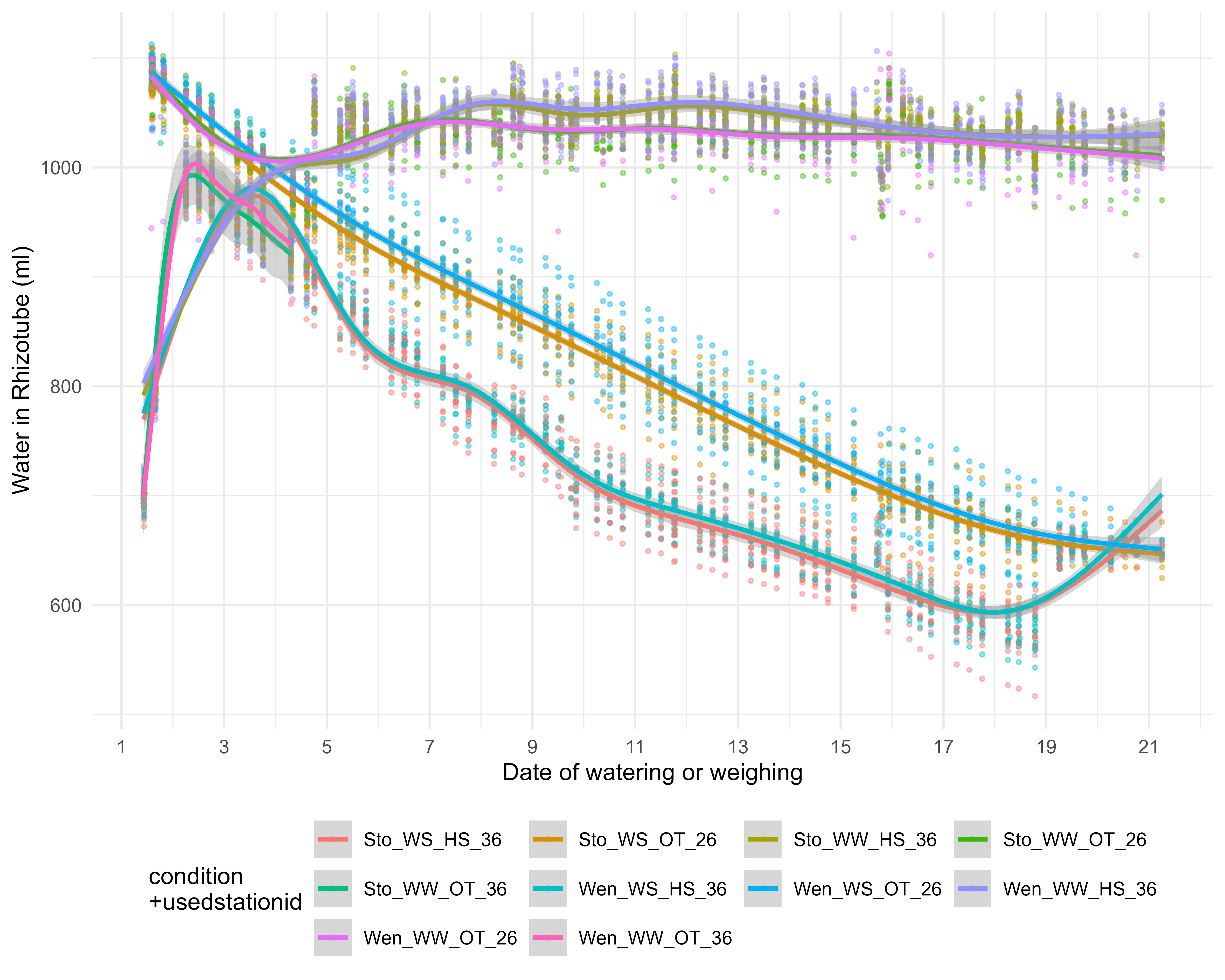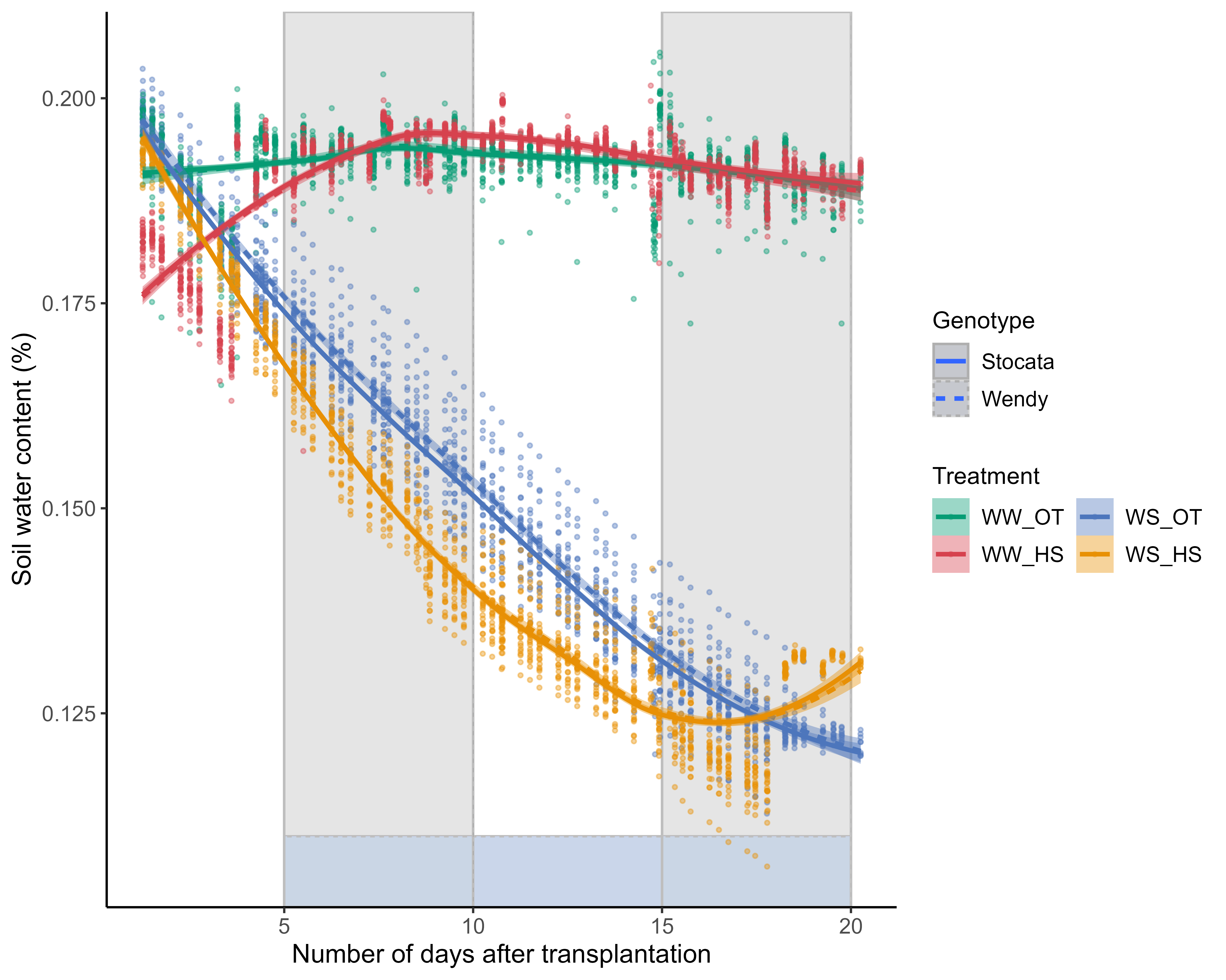{#fig-water_content}- Find the date of the next measurement for the same rizotube. Attention the last measurement is deleted.## Evapotranspiration### Kinetics::: callout-caution*Be careful, this step takes a lot of time This step also adds a night day column and a night morning and afternoon column. This part also measures the time between two weighings*:::```{r evapotranspiration, eval=F}# /!\ take time 5 min at leastcat_col("Caution: you have to wait a long time here", "red")global_weight_select3=read.csv("data/water/weighing_watering_output/global_weight_select3.csv")[-1]global_weight_select3$next_weight=NAlevels_factor_plant_id=levels(as.factor(global_weight_select3$plant_id))pb = txtProgressBar(min = 0, max = length(levels_factor_plant_id), initial = 0,style=3)#progresse bar for (i in levels_factor_plant_id){ setTxtProgressBar(pb,match(i,levels_factor_plant_id)) #progresse bar data_watering_select_x=global_weight_select3 %>% filter(plant_id==i) %>% arrange(resultdate_time) levels_factor_resultdate_time=data_watering_select_x$resultdate_time for (j in 1:length(levels_factor_resultdate_time)){ for (k in 1:length(global_weight_select3$studyname)){ if(as.character(global_weight_select3$plant_id[k])==i){ # print(data_watering_select$plantid[k]) if(global_weight_select3$resultdate_time[k]==levels_factor_resultdate_time[j]){ global_weight_select3$next_weight[k]=as.character(levels_factor_resultdate_time[j+1]) #print(paste(i,levels_factor_resultdate_time[j],levels_factor_resultdate_time[j+1], sep="_")) } } } }}df_evapotranspi=global_weight_select3 %>% drop_na(next_weight)df_evapotranspi$water_after=NApb = txtProgressBar(min = 0, max = length(df_evapotranspi$studyname), initial = 0,style=3)#progresse bar for (i in 1:length(df_evapotranspi$studyname)){ for (j in 1:length(global_weight_select3$studyname)){ if(df_evapotranspi$plant_id[i]==global_weight_select3$plant_id[j]){ if (df_evapotranspi$next_weight[i]==global_weight_select3$resultdate_time[j]){ df_evapotranspi$water_after[i]=global_weight_select3$water_in_rt[j] } } } setTxtProgressBar(pb,i) #progresse bar}df_evapotranspi$evapotranspiration=df_evapotranspi$water_in_rt-df_evapotranspi$water_after+df_evapotranspi$deliveredquantity#diff time enter the two weightdf_evapotranspi$diff_resultdate_time=as.POSIXct(df_evapotranspi$next_weight)-as.POSIXct(df_evapotranspi$resultdate_time)#transforme date time of next_weight in juste time for separate by morning afternoone nightdf_evapotranspi$next_weight_time=format(strftime(df_evapotranspi$next_weight, format = "%H:%M:%S"))df_evapotranspi$night_day=NApb = txtProgressBar(min = 0, max = length(df_evapotranspi$studyname), initial = 0,style=3)#progresse bar for (i in seq_along(df_evapotranspi$studyname)){ if (format(strftime(df_evapotranspi$next_weight[i], format = "%H:%M:%S"))<format(strftime("2021-10-01 09:18:00", format = "%H:%M:%S"))){ if (format(strftime(df_evapotranspi$resultdate_time[i], format = "%H:%M:%S"))>format(strftime("2021-10-01 17:00:00", format = "%H:%M:%S"))){ # print(paste(data_watering_select_transpiration_select$time[i],data_watering_select_transpiration_select$next_weight_time[i],sep="_")) df_evapotranspi$night_day[i]="night" }else{ df_evapotranspi$night_day[i]="day" } }else{ df_evapotranspi$night_day[i]="day" } setTxtProgressBar(pb,i) #progresse bar }df_evapotranspi$morning_afternoon="night"pb = txtProgressBar(min = 0, max = length(df_evapotranspi$studyname), initial = 0,style=3) #progresse bar for (i in seq_along(df_evapotranspi$studyname)){ if(df_evapotranspi$night_day[i]=="day"){ if(format(strftime(df_evapotranspi$resultdate_time[i], format = "%H:%M:%S"))<format(strftime("2021-10-01 11:00:00", format = "%H:%M:%S"))){ df_evapotranspi$morning_afternoon[i]="morning" }else(df_evapotranspi$morning_afternoon[i]="afternoon") } setTxtProgressBar(pb,i) #progresse bar }write.csv(df_evapotranspi,here::here("data/water/weighing_watering_output/df_evapotranspi.csv"))```- Plot exemple for *RT1067*```{r evapotranspiration2,fig.cap="Evapotranspiration for one plante of the RT 1067 (ml) between two watering or weighing",fig.height=5, eval=F}df_evapotranspi=read.csv(here::here("data/water/weighing_watering_output/df_evapotranspi.csv"))[-1]df_evapotranspi$resultdate_time=as.POSIXct(df_evapotranspi$resultdate_time)plot_x=df_evapotranspi %>% filter(plant_id=="1069")%>% ggplot(aes(x=resultdate_time, y=evapotranspiration/2, colour=paste0(condition,"_",usedstationid), group=c(paste0(condition,"_",usedstationid)))) + geom_smooth(se=F)+ geom_point()+ scale_x_datetime(breaks=("1 day"), minor_breaks=("1 hour"),labels = date_format("%b-%d %H:%M:%S"))+ labs(x="Date and time", y="Evapotranspiration for one plante of one \n rhizotube (ml) between two watering or weighing",color="condition \n+usedstationid")+ theme_minimal()+ theme(axis.text.x = element_text(angle = 90, hjust = 1)) + theme(legend.position="bottom")ggsave(here::here("report/water/plot/evapotranspiration_1069.svg"), plot_x, width = 20,height = 16, units = "cm")```(plot/water/evapotranspiration_1069.svg)```{r summury of the data, eval=F}sum_by_date=aggregate(df_evapotranspi$evapotranspiration, by=list(df_evapotranspi$plant_id, df_evapotranspi$condition,df_evapotranspi$resultdate,df_evapotranspi$genotype,df_evapotranspi$heat_condition), FUN=sum)``````{r plotresumsum, fig.cap="Evapotranspiration for one plante of one rhizotube (ml) during on day",fig.height=7, eval=F}plot_x=sum_by_date %>% mutate(Group.1=factor(Group.1,levels=c("Sto_WW_OT","Sto_WW_HS","Sto_WS_OT","Sto_WS_HS","Wen_WW_OT","Wen_WW_HS","Wen_WS_OT","Wen_WS_HS"))) %>% ggplot(aes(x=as.factor(Group.3),y=x/2,fill=Group.2))+ geom_boxplot(outlier.alpha = 0)+ #facet_grid(Group.5~.)+ #geom_point(position=position_jitterdodge(),alpha=0.3)+ theme(axis.text.x = element_text(angle = 90, vjust = 0.5, hjust=1))+ scale_fill_manual(values=manu_palett)+ labs(x="Date", y="Evapotranspiration for one plante of one rhizotube (ml) during on day")+ theme(legend.position="bottom")ggsave(here::here("report/water/plot/evapotranspiration_each_plant.svg"), plot_x, width = 20,height = 16, units = "cm")```- Error detection```{r withResultdatetime, fig.height=9, fig.width = 8,fig.cap= "Frequency and date of evapotranspiration for a plant between two waterings", eval=F}plot_x<- df_evapotranspi %>% mutate(condition=factor(condition,levels=c("Sto_WW_OT","Sto_WW_HS","Sto_WS_OT","Sto_WS_HS","Wen_WW_OT","Wen_WW_HS","Wen_WS_OT","Wen_WS_HS"))) %>% ggplot(aes(x=as.POSIXct(format(as.POSIXct(resultdate_time),format = "%H:%M:%S"),format = "%H:%M:%S"),y=evapotranspiration/2,col=condition))+ geom_point()+ facet_wrap(~resultdate)+ scale_color_manual(values=manu_palett)+ theme(axis.text.x = element_text(angle = 90, vjust = 0.5, hjust=1))+ labs(y="Evapotranspiration between two weighings (ml) for one plant", x="Date time")+ theme(legend.position="bottom")ggsave(here::here("report/water/plot/find_error_evapo.svg"), plot_x, width = 20,height = 18, units = "cm")```Sometimes have less than three waterings per day and at different times or more than 3. This can lead to calculation errors later on the script.```{r ErrorTiming, fig.cap="Error in data collection for some Rhizotubes", fig.height=9, fig.width = 8, eval=F}plot_x<- df_evapotranspi %>% mutate(condition=factor(condition,levels=c("Sto_WW_OT","Sto_WW_HS","Sto_WS_OT","Sto_WS_HS","Wen_WW_OT","Wen_WW_HS","Wen_WS_OT","Wen_WS_HS"))) %>% ggplot(aes(x=as.POSIXct(format(as.POSIXct(resultdate_time),format = "%H:%M:%S"),format = "%H:%M:%S"),y=diff_resultdate_time/60,col=condition))+ labs(y="Time (hours) between two weighing measurements for each rhizotube", x="Date and time")+ geom_point()+ facet_wrap(~resultdate)+ scale_color_manual(values=manu_palett)+ theme(axis.text.x = element_text(angle = 90, vjust = 0.5, hjust=1))+ theme(legend.position="bottom")ggsave(here::here("report/water/plot/find_error_evapo_time_between.svg"), plot_x, width = 20,height = 18, units = "cm")```**Why do I have the RT 1035 which has such a huge value between two waterings?** Because there are missing values for the 1035 between the 27th at 7:45 and the 29th at 12:06. On the 27th the measurements of 14:27, 18:05 and 20:30 are missing. On the 28th the data of 6:06, 12:05 and 18:05 and on the 29th the data of 6:06.Division of the evapotranspiration by the time between two weighing measurements. That is, divide by the weight after watering minus the weight before watering.```{r DivEvapo2,fig.cap="Evapotranspiration of a plant per rhizotube ml.hour1", fig.height=9, fig.width = 8, eval=F}#if i divide one by onedf_evapotranspi$div=df_evapotranspi$evapotranspiration/(as.numeric(df_evapotranspi$diff_resultdate_time)/60)plot_x<- df_evapotranspi %>% mutate(condition=factor(condition,levels=c("Sto_WW_OT","Sto_WW_HS","Sto_WS_OT","Sto_WS_HS","Wen_WW_OT","Wen_WW_HS","Wen_WS_OT","Wen_WS_HS"))) %>% filter(div>-1) %>% ggplot(aes(x=as.POSIXct(format(as.POSIXct(resultdate_time),format = "%H:%M:%S"),format = "%H:%M:%S"),y=div/2,col=condition))+ geom_point(size=1.2, alpha=.5)+ labs(y=expression(paste("Evapotranspiration of a plant per rhizotube (ml.",hour^{-1},")")), x="Date and time")+ facet_wrap(~resultdate)+ scale_color_manual(values=manu_palett)+ theme(axis.text.x = element_text(angle = 90, vjust = 0.5, hjust=1))+ theme(legend.position="bottom")ggsave(here::here("report/water/plot/evapo_by_plant_per_RT.svg"), plot_x, width = 22,height = 18, units = "cm")```Then I remove some aberrant data or that could bother me for the calculations. I remove the values of 2021-09-24 because the last weighing was done at 15h. I also remove the time between two weighing more than 16h30 and finally I remove the results of rhizotube 3 (aberrant results).If I separate the evaporation between day and night. If I separate the evapotranspiration between day and night. One can see logically that evapotranspiration is much lower at night than during the day. During the day and in the course of the experiment, there is an increasing increase in evapotranspiration for plants in well-watered conditions. During the day, and during the first heat wave (from day X to day X), evapotranspiration increases for both genotypes, and then returns to a state close to the one observed in plants in optimal temperature conditions. During the second heat wave (from day X to day X), during the day and in well-watered conditions, there could be have a difference between the two genotypes. Wendy could be have a higher evapotranspiration in this condition. Can this be explained by their different aerial and root architecture (for the same biomass)? Towards the end we can see the re-watering of the plants in stressed condition.```{r plotnightday,fig.height=7, echo=F,fig.cap="Evapotranspiration of a plant per rhizotube ml.hour1 in the night and in the day", eval=F}df_evapotranspi2=df_evapotranspi %>% filter(as.Date(resultdate)>as.Date("2021-09-24")) %>% #because the 2021-09-24 the last weight was one 15h filter(diff_resultdate_time<1000) %>% filter(plant_id != "3") %>% mutate(condition=factor(condition,levels=c("Sto_WW_OT", "Sto_WW_HS", "Sto_WS_OT", "Sto_WS_HS", "Wen_WW_OT", "Wen_WW_HS", "Wen_WS_OT", "Wen_WS_HS"))) df_evapotranspi2$night_day[df_evapotranspi2$night_day == "day"] <- "Day" df_evapotranspi2$night_day[df_evapotranspi2$night_day == "night"] <- "Night"Fig1=ggarrange(df_evapotranspi2 %>% mutate(climat_condition=paste(sep="_",water_condition,heat_condition)) %>% mutate(condition=factor(condition,levels=c("Sto_WW_OT","Sto_WW_HS","Sto_WS_OT","Sto_WS_HS","Wen_WW_OT","Wen_WW_HS","Wen_WS_OT","Wen_WS_HS"))) %>% mutate(climat_condition=factor(climat_condition,levels=c("WW_OT","WS_OT","WW_HS","WS_HS"))) %>% filter(div<20) %>% ggplot(aes(x=(as.POSIXct(resultdate_time)-as.POSIXct("2021-09-22 00:00:00")),y=div/2,col=climat_condition,fill=climat_condition,linetype=genotype))+ #geom_rect(aes(xmin=as.POSIXct('2021-10-07 00:00:00'),xmax = as.POSIXct('2021-10-11 00:00:00'), ymin = -Inf,ymax = Inf), fill = 'pink', alpha = 0.05)+ #geom_rect(aes(xmin=as.POSIXct('2021-09-27 00:00:00'),xmax = as.POSIXct('2021-10-02 00:00:00'), ymin = -Inf,ymax = Inf), fill = 'pink', alpha = 0.05)+ geom_rect(xmin = 5, xmax = 20, ymin = -Inf, ymax = -1, fill = "#c9d5ea", alpha = 0.5,col="gray") + geom_rect(xmin = 5, xmax = 10, ymin = -Inf, ymax = Inf, fill = "lightgray", alpha = 0.02,col="gray") + geom_rect(xmin = 15, xmax = 20, ymin = -Inf, ymax = Inf, fill = "lightgray", alpha = 0.02,col="gray") + facet_grid(~night_day)+ geom_point(alpha = 0.2,size=.7)+ scale_color_manual(values=climate_pallet)+ scale_fill_manual(values=climate_pallet)+ geom_smooth(alpha=0.2)+ labs(y=expression(paste("Evapotranspiration by plant (ml.",hour^{-1},")")), x="Number of days afters transplantation")+ theme(axis.text.x = element_text(angle = 90, vjust = 0.5, hjust=1))+ theme(legend.position="right")+ labs(color="Treatment",fill="Treatment",linetype="Genotype")+ my_theme#+ #scale_x_datetime(date_breaks= "2 days", date_minor_breaks = "12 hour")+ #scale_y_continuous(breaks=1))#Fig1# # png(here::here("water/plot/evapotranspi_genotype.png"), width = 29.7, height = 21, units = 'cm', res = 600)# Fig1# dev.off()write.csv(x = df_evapotranspi2 %>% dplyr::select(plant_id, plant_num, condition, resultdate_time, div,humidity) %>% mutate(div=div/2) %>% dplyr::rename(evapotranspiration_rate_plant=div) %>% dplyr::rename(water_content=humidity), file = here::here("data/water/weighing_watering_output/evapotranspiration_plant_day_night.csv"),row.names = F)# ggsave(here::here("report/water/plot/evapotranspi_genotype_day_night.svg"), # grid.arrange (Fig1), width = 22,height = 18, units = "cm")```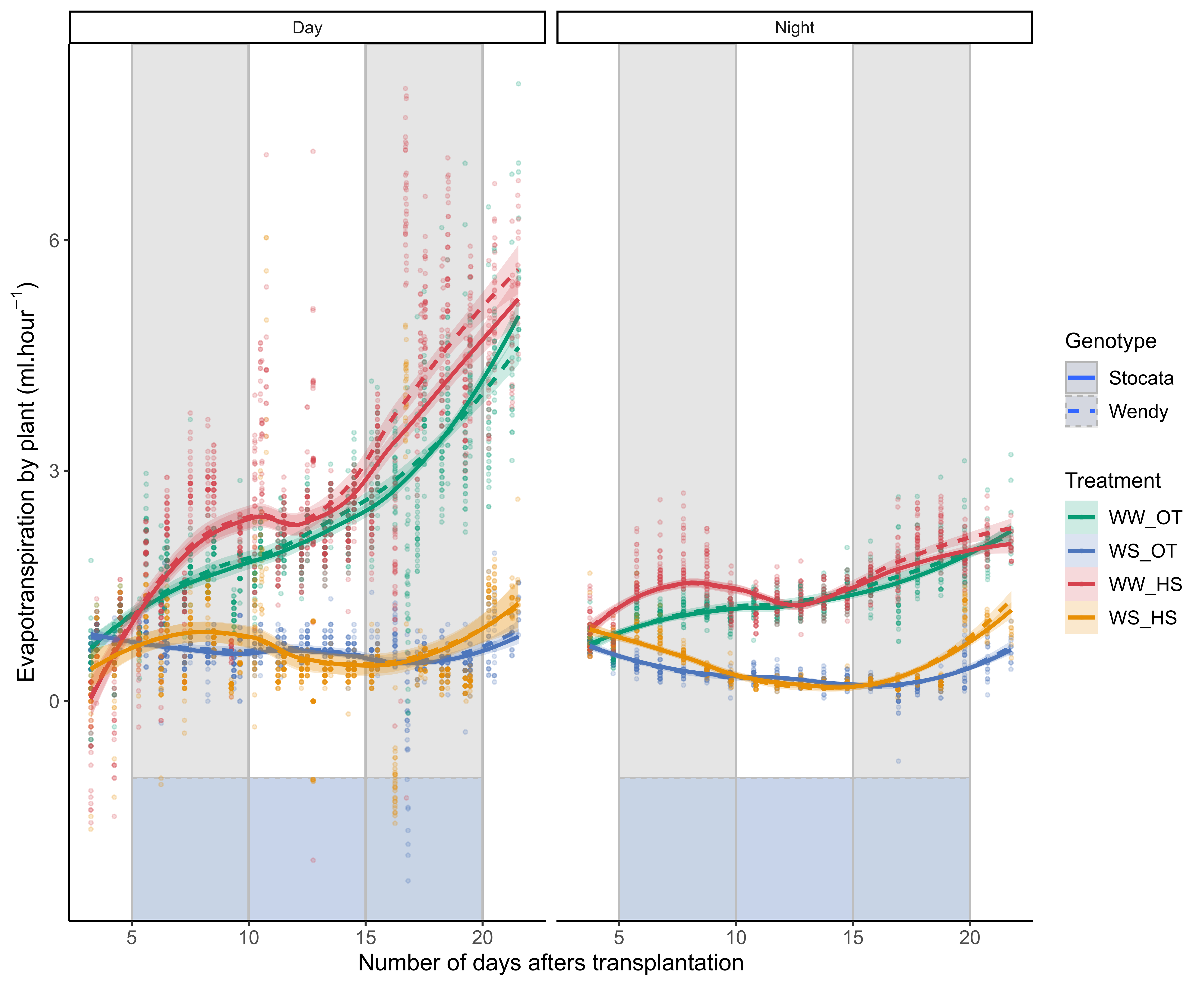{#fig-evapotranspiration}If we look at the differences between conditions for each period of the day (morning, afternoon, evening) but not in ml.hours but in cumulative. There does not seem to be any major difference in evapotranspiration between these three periods.```{r plotnightDayAfternnonNight,fig.height=10,fig.width=7, echo=F,fig.cap="Cumul of evapotranspiration of a plant per rhizotube ml.hour1", eval=F}sum_by_date_night_morning_afternoon=df_evapotranspi2 %>% group_by(plant_id, condition ,resultdate,genotype,water_condition,heat_condition ,morning_afternoon)%>% dplyr::summarise(.groups = 'drop',sum_evapotranspiration = sum(evapotranspiration), n_evapotranspiration = length(evapotranspiration),sum_diff_resultdate_time = sum(diff_resultdate_time)) %>% mutate(div_night_day=sum_evapotranspiration/(as.numeric(sum_diff_resultdate_time)/60))plot_x<-sum_by_date_night_morning_afternoon %>% #filter(water_condition=="WW") %>% ggplot(aes(x=resultdate,y=sum_evapotranspiration/2,fill=condition))+ geom_rect(aes(xmin='2021-09-27',xmax = '2021-10-02', ymin = -Inf,ymax = Inf), fill = 'pink', alpha = 0.05)+ geom_rect(aes(xmin='2021-10-07',xmax = '2021-10-11', ymin = -Inf,ymax = Inf), fill = 'pink', alpha = 0.05)+ geom_boxplot(outlier.alpha = 0)+ #geom_point(position=position_jitterdodge(),alpha=0.3)+ theme(axis.text.x = element_text(angle = 90, vjust = 0.5, hjust=1))+ scale_fill_manual(values=manu_palett)+ facet_grid(morning_afternoon~.)+ ylab('Evapotranspiration (cumul ml in the day per RT) by plant by periode of the day ')+ theme(legend.position="bottom")ggsave(here::here("report/water/plot/evapotranspi_genotype_morning_afternoon_night.svg"), plot_x, width = 22,height = 18, units = "cm")```### Total evapotranspiration```{r TotalEvapotranspiration, fig.height=6 ,fig.cap="Total cumul of evapotranspiration per plant per condition ml hour 1",results="hide", eval=F}df_evapotranspi3=merge( df_evapotranspi2, read.csv2(here::here("data/physio/global_physio.csv")) %>% dplyr::select(plant_id,weight_root, leaf_area,sum_biomass), by="plant_id", all = T)write.csv(df_evapotranspi3, here::here("data/water/weighing_watering_output/df_evapo3.csv"))#mean of harvest 1#sum evapotransipration by plant_idsum_evapo_end=df_evapotranspi3 %>% group_by(plant_id, condition, recolte) %>% dplyr::summarise(.groups = 'drop',sum_total_evapotranspiration=sum(evapotranspiration)) %>% drop_na(sum_total_evapotranspiration)## write result evapotranspi3write.csv(sum_evapo_end,here::here("data/water/weighing_watering_output/sum_evapotranspi.csv"))sum_evapo_end_1=sum_evapo_end %>% filter(recolte==1)sum_evapo_end_2=sum_evapo_end %>% filter(recolte==2) %>% mutate(condition=factor(condition,levels=c("Sto_WW_OT","Sto_WS_OT","Sto_WW_HS","Sto_WS_HS","Wen_WW_OT","Wen_WS_OT","Wen_WW_HS","Wen_WS_HS")))# # plot_x=stat_analyse(# data=sum_evapo_end_1 %>% # data.frame() %>% # mutate(condition=factor(condition,levels=c("Sto_WW_OT","Sto_WS_OT","Sto_WW_HS","Sto_WS_HS","Wen_WW_OT","Wen_WS_OT","Wen_WW_HS","Wen_WS_HS"))),# column_value = "sum_total_evapotranspiration",# category_variables = "condition",# grp_var = "",# show_plot = T,# outlier_show = F, # label_outlier = "plant_id",# biologist_stats = T,# Ylab_i = "Total evaporation of plants from harvest 1 before harvest (ml)"# )# # plot_x[["plot"]]+# labs(color=NULL,fill=NULL,subtitle = df_alpha_info$for_title[i])+# theme (axis.ticks.x = element_blank(),# Masquer les ticks de l'axe x# axis.text.x=element_blank (),# axis.title.x = element_blank(),# legend.position = "none",# plot.subtitle = element_text(face = "bold"),# plot.caption = element_blank()# ) p1=Plettre_modif( Z=sum_evapo_end_1, X=sum_evapo_end_1$condition, Y=sum_evapo_end_1$sum_total_evapotranspiration/2, Xlab = "Condition", Ylab = "Total evaporation of plants from harvest 1 before harvest (ml)", Y_bis = "sum_total_evapotranspiration", Tukey=T, outlier_show = F, label_outlier = "plant_id")p1=p1[[1]]p2=Plettre_modif( Z=sum_evapo_end_2, X=sum_evapo_end_2$condition, Y=sum_evapo_end_2$sum_total_evapotranspiration/2, Xlab = "Condition", Ylab = "Total evaporation of plants before harvest 2 (ml)", Y_bis = "sum_total_evapotranspiration", Tukey=T, outlier_show = F, label_outlier = "plant_id")p2=p2[[1]]#plot_grid(p1, p2, ncol = 2, nrow = 1)ggsave(here::here("report/water/plot/total_evapotranspi.svg"), plot_grid(p1, p2, ncol = 2, nrow = 1), width = 22,height = 18, units = "cm")```## WUE and sRWU Since we have chosen to make correlations between variables measured by plant and the efficiencies of water, element, radiation ... we have chosen to make averages on the first harvest and to make calculations with these averages (H1) vs harvest 2 (HS).```{r ResumData, eval=T}df_use_for_WUE=merge( read.csv(here::here("data/water/weighing_watering_output/df_evapo3.csv")) %>% drop_na(evapotranspiration)%>% drop_na(sum_biomass), as.data.frame(read.csv(here::here("data/water/weighing_watering_output/df_evapo3.csv")) %>% group_by(plant_id, condition, recolte) %>% dplyr::summarise(.groups = 'drop',sum_total_evapotranspiration=sum(evapotranspiration)) %>% drop_na(sum_total_evapotranspiration)) %>% dplyr::select(plant_id,sum_total_evapotranspiration ) %>% drop_na(sum_total_evapotranspiration), all=T, by="plant_id") %>% group_by(recolte,condition)%>% dplyr::summarise(mean_sum_biomass =mean(sum_biomass), mean_sum_total_evapotranspiration=mean(sum_total_evapotranspiration),.groups = 'drop') %>% #.groups = 'drop' for delet warning message drop_na(mean_sum_biomass) %>% as.data.frame() %>% mutate(mean_sum_biomass=mean_sum_biomass*1000) %>% mutate(mean_sum_total_evapotranspiration=mean_sum_total_evapotranspiration/2)kbl(df_use_for_WUE, caption = "Resume of the data use for Water Use Efficiency (WUE) for eatch condition",col.names=c("Harvest","Condition", "Average total weight (mg)", "Average total evapotranspiration (ml)"),digits = 1) %>% kable_paper(full_width = F) %>% #column_spec(3, color = "white",background = spec_color(WUE$mean_sum_biomass, end = 0.7))%>% column_spec(4, color = "white",background = spec_color(df_use_for_WUE$mean_sum_biomass, end = 0.7))```### WUE with mean in H1 and H2Water Use Efficiency, Thesis Couchoud (p69): Stomata closure may not be complete, transpiration is then more reduced than the net assimilation of atmospheric CO2 by photosynthesis. An increase in water use efficiency (WUE) is then observed (Maury et al., 2011). This change in WUE in response to water stress has been reported in multiple studies and high WUE is commonly associated with better tolerance to water stress (Chaves et al., 2003, 2009; Siopongco et al., 2006; Xu et al., 2010; Anjum et al., 2011; Erice et al., 2011).Water Use Efficiency (WUE) between date t1 and t2 was calculated as the ratio of the plant biomass (BM) accumulated over the amount of water evapotranspirated by the plant during this period (QH2O) and is expressed in g. gH2O-1:```{r WUE, eval=F}# Process to calculWUE2mean=df_use_for_WUEWUE2mean$result_WUE=NAfor (i in 1:nrow(WUE2mean)){ for (j in 1:nrow(WUE2mean)){ if (WUE2mean$recolte[i]==1){ WUE2mean$result_WUE[i]=NA }else if (WUE2mean$recolte[i]==2 && WUE2mean$recolte[j]==1){ if(str_sub(WUE2mean$condition[i], 1, 3)==str_sub(WUE2mean$condition[j], 1, 3)){ WUE2mean$result_WUE[i]=(WUE2mean$mean_sum_biomass[i]/1000-WUE2mean$mean_sum_biomass[j]/1000)/(((WUE2mean$mean_sum_total_evapotranspiration[i]/1000))-((WUE2mean$mean_sum_total_evapotranspiration[j]/1000))) } } }}write.csv(WUE2mean,here::here("data/water/weighing_watering_output/WUE_with_mean_h1_and_mean_h2.csv"))``````{r, eval=T}# show tableread.csv(here::here("data/water/weighing_watering_output/WUE_with_mean_h1_and_mean_h2.csv")) %>%dplyr::select(recolte,condition,mean_sum_biomass, mean_sum_total_evapotranspiration, result_WUE) %>%mutate(mean_sum_biomass=mean_sum_biomass/1000,mean_sum_total_evapotranspiration=(mean_sum_total_evapotranspiration/1000),result_WUE=result_WUE) %>%kbl(caption = "WUE for eatch condition. Only mean using",col.names=c("Harvest","Condition", "Dry weight total (g)", "Sum of the evapotranspiration (L)", "WUE (g. L H20-1)"), digits = 2) %>% kable_paper(full_width = F) %>%column_spec(5, color = "white",background = spec_color(read.csv(here::here("data/water/weighing_watering_output/WUE_with_mean_h1_and_mean_h2.csv")) %>% pull(result_WUE), end = 0.7))```### WUE and sRWU (H1 mean )```{r, eval=F}# Data importation and preparation for H1 and H2df_H1_mean<-merge(sum_evapo_end %>% filter(recolte==1),read.csv2(here::here("data/physio/global_physio.csv")) %>% dplyr::select(plant_id, weight_root,sum_biomass, plant_num,genotype,date_recolte,recolte) %>% filter(recolte==1) %>% dplyr::select(-recolte),by="plant_id", all=T) %>% drop_na(weight_root,sum_total_evapotranspiration) %>% mutate(sum_total_evapotranspiration=sum_total_evapotranspiration/1000/2) %>% dplyr::group_by(condition, genotype,recolte,date_recolte) %>% dplyr::summarise(across(sum_total_evapotranspiration:sum_biomass, ~ mean(.x, na.rm = TRUE))) %>% dplyr::rename_all(~ paste0(., "_H1")) %>% dplyr::rename(genotype=genotype_H1)df_H2<-merge(sum_evapo_end %>% filter(recolte==2),read.csv2(here::here("data/physio/global_physio.csv")) %>% dplyr::select(plant_id, weight_root,sum_biomass, plant_num,genotype,date_recolte,recolte) %>% filter(recolte==2) %>% dplyr::select(-recolte),by="plant_id", all=T) %>% drop_na(weight_root,sum_total_evapotranspiration) %>% mutate(sum_total_evapotranspiration=sum_total_evapotranspiration/1000/2) %>% dplyr::rename_all(~ paste0(., "_H2")) %>% dplyr::rename(genotype=genotype_H2)# Process WUE and sRWUWUE_sRWU_1mean=full_join(df_H2, df_H1_mean, by="genotype",relationship = "many-to-many") %>% mutate(WUE=(sum_biomass_H2 -sum_biomass_H1)/(sum_total_evapotranspiration_H2 -sum_total_evapotranspiration_H1)) %>% mutate(sRWU=(sum_total_evapotranspiration_H2-sum_total_evapotranspiration_H1)/ (( (as.numeric(as.Date(date_recolte_H2)-as.Date(date_recolte_H1))) * ((weight_root_H2+weight_root_H1)/2) ))) %>% dplyr::rename(condition=condition_H2) %>% mutate(water_condition=str_sub(condition, 5, 6)) %>% mutate(heat_condition=str_sub(condition, 8, 9)) %>% mutate(climat_condition=paste0(water_condition, "_", heat_condition)) %>% mutate(condition=factor(condition,levels=c("Sto_WW_OT","Sto_WS_OT","Sto_WW_HS","Sto_WS_HS","Wen_WW_OT","Wen_WS_OT","Wen_WW_HS","Wen_WS_HS"))) %>% mutate(climat_condition=factor(climat_condition,levels=c("WW_OT","WS_OT","WW_HS","WS_HS")))# export resultswrite.csv(WUE_sRWU_1mean,here::here(paste(sep="_","data/water/weighing_watering_output/WUE_sRWU_1mean.csv")))# Show resultspWUE=stat_analyse(data =WUE_sRWU_1mean, column_value = "WUE", category_variables = c("climat_condition"), grp_var = "genotype", control_conditions = c("WW_OT"), biologist_stats = T, strip_normale = F, outlier_show = F, label_outlier = "plant_num_H2", show_plot = T, hex_pallet = climate_pallet, Ylab_i = paste0("Water Use Efficiency (g/L)") )pWUE<-pWUE[["plot"]]+labs(color="Treatment",fill="Treatment")+ theme(axis.title.x=element_blank(), axis.text.x=element_blank(), panel.grid.major = element_blank(), panel.grid.minor = element_blank(), axis.ticks.x = element_blank() )+labs(subtitle = "WUE with one mean")# Show resultspsRWU=stat_analyse(data =WUE_sRWU_1mean, column_value = "sRWU", category_variables = c("climat_condition"), grp_var = "genotype", control_conditions = c("WW_OT"), biologist_stats = T, strip_normale = F, outlier_show = F, label_outlier = "plant_num_H2", show_plot = T, hex_pallet = climate_pallet, Ylab_i = paste0("specific Root Water Uptake (gH2O[gBMroot day-1]-1)") )psRWU<-psRWU[["plot"]]+labs(color="Treatment",fill="Treatment")+ theme(axis.title.x=element_blank(), axis.text.x=element_blank(), panel.grid.major = element_blank(), panel.grid.minor = element_blank(), axis.ticks.x = element_blank() )+labs(subtitle = "sRWU with one mean")combined_plot<-(pWUE+psRWU) + plot_layout(guides = 'collect')# export figurepng(here::here(paste0("report/water/plot/WUE_sRWU_1mean.png")), width = 18, height = 10, units = 'cm', res = 900)combined_plotdev.off()```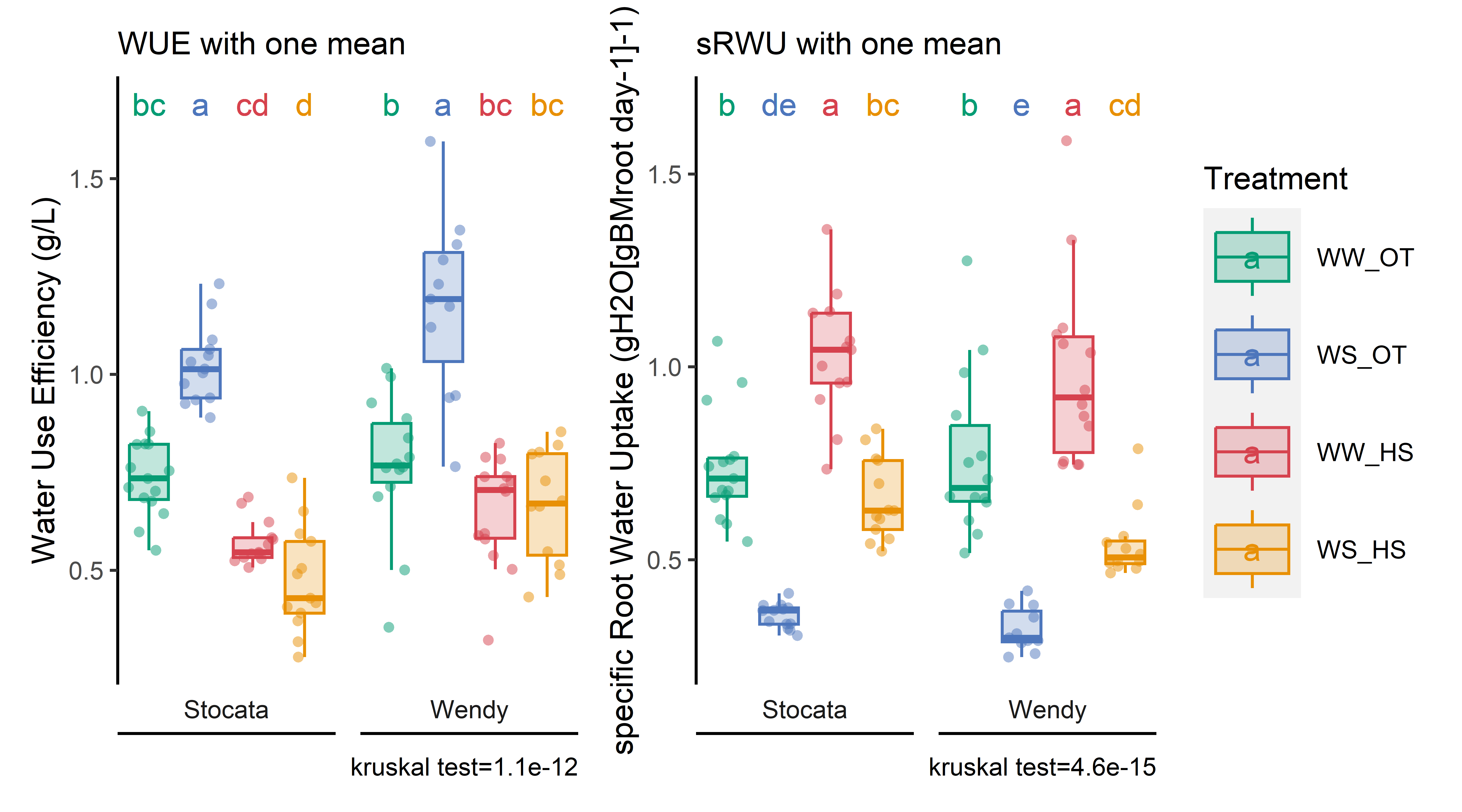```{r}# show tableread.csv(here::here("data/water/weighing_watering_output/WUE_sRWU_1mean.csv")) %>%dplyr::select(condition, WUE,sRWU) %>% dplyr::group_by(condition) %>% dplyr::summarise(across(WUE:sRWU, mean, na.rm =TRUE)) %>%kbl(caption ="WUE and sRWU for eatch condition. Mean only for H1", col.names=c("Condition", "WUE (g. L H20-1)","sRWU(gH2O[gBMroot day-1]-1)"), digits =2) %>%kable_paper(full_width = F) %>%column_spec(2, color ="white",background =spec_color(read.csv(here::here("data/water/weighing_watering_output/WUE_sRWU_1mean.csv")) %>%dplyr::group_by(condition) %>% dplyr::summarise(across(WUE:sRWU, mean, na.rm =TRUE)) %>%pull(WUE), end =0.7)) %>%column_spec(3, color ="white",background =spec_color(read.csv(here::here("data/water/weighing_watering_output/WUE_sRWU_1mean.csv")) %>%dplyr::group_by(condition) %>%dplyr::summarise(across(WUE:sRWU, mean, na.rm =TRUE)) %>%pull(sRWU), end =0.7))```### WUE and sRWU (Drawing with discount )Now according to Marion, I have to do random draw for statistical analysis *see script used for nodosity in my first paper*. I have a repetition of the draw of 100 for eatch condition according to Denis Vile. The problem is that I have lots of data warning of different df. Already only one measurement for root weight. So I have to halve the evapotranspiration because I don't know which RT plant it is.```{r, eval=F}# Data generationdf_WUE_sRWU_bootstrap=merge(sum_evapo_end,read.csv2(here::here("data/physio/global_physio.csv")) %>% dplyr::select(plant_id, weight_root,sum_biomass, plant_num,genotype,date_recolte),by="plant_id", all=T ) %>% drop_na(weight_root,sum_total_evapotranspiration) %>% mutate(sum_total_evapotranspiration=sum_total_evapotranspiration/1000/2)# Process to bootstraplist_condition<-levels(as.factor(df_WUE_sRWU_bootstrap$condition))### parameter rep=100set.seed(1)df_bootstrap=data.frame()#For eatch condition of the harvest 2for (i in 1:rep){ for (cond_x in list_condition){ df_x=df_WUE_sRWU_bootstrap %>% filter(recolte=="2") %>% filter(condition==cond_x) df_x_taking=df_x %>% filter(plant_num==sample(df_x$plant_num,1,replace=T)) if(str_sub(df_x_taking$condition, 1, 3)=="Sto"){ df_y=df_wue %>% filter(recolte=="1") %>% filter(genotype=="Stocata") }else { df_y=df_wue %>% filter(recolte=="1") %>% filter(genotype=="Wendy") } df_y_taking=df_y %>% filter(plant_num==sample(df_y$plant_num,1,replace=T)) colnames(df_x_taking)=c("plant_id_rec_2","condition","recolte_2","sum_evapo_transpi_2","weight_root_2","weight_tot_2","plant_num_2","genotype_2","date_recolte_2") colnames(df_y_taking)=c("plant_id_rec_1","condition1","recolte_1","sum_evapo_transpi_1","weight_root_1","weight_tot_1","plant_num_1","genotype_1","date_recolte_1") df_bind=cbind(df_y_taking,df_x_taking) df_bind$rep=i df_bind$simulation=paste0(i,"_",cond_x) df_bind$WUE=(df_bind$weight_tot_2-df_bind$weight_tot_1)/(df_bind$sum_evapo_transpi_2-df_bind$sum_evapo_transpi_1) df_bind$sRWU=(df_bind$sum_evapo_transpi_2-df_bind$sum_evapo_transpi_1)/ (( (as.numeric(as.Date(df_bind$date_recolte_2)-as.Date(df_bind$date_recolte_1))) * ((df_bind$weight_root_2+df_bind$weight_root_1)/2) )) #print(str_sub(df_x_taking$condition, 1, 3)) df_bootstrap=rbind(df_bootstrap,df_bind) } fit <- aov(WUE ~ condition, df_compile)# analyse de varianceprint(summary(fit)[[1]][["Pr(>F)"]][1]) ; }# Obviously the more loops i make the stronger i am !!! df_bootstrap=df_bootstrap %>% mutate(water_condition=str_sub(condition, 5, 6)) %>% mutate(heat_condition=str_sub(condition, 8, 9)) %>% mutate(climat_condition=paste0(water_condition, "_", heat_condition)) %>% mutate(condition=factor(condition,levels=c("Sto_WW_OT","Sto_WS_OT","Sto_WW_HS","Sto_WS_HS","Wen_WW_OT","Wen_WS_OT","Wen_WW_HS","Wen_WS_HS"))) %>% mutate(climat_condition=factor(climat_condition,levels=c("WW_OT","WS_OT","WW_HS","WS_HS"))) %>% dplyr::rename(genotype=genotype_2)# export resultswrite.csv(df_bootstrap,here::here(paste(sep="_","data/water/weighing_watering_output/WUE_sRWU_Bootstrap.csv")))# Show resultspWUE=stat_analyse(data =df_bootstrap, column_value = "WUE", category_variables = c("climat_condition"), grp_var = "genotype", control_conditions = c("WW_OT"), biologist_stats = T, strip_normale = F, outlier_show = F, label_outlier = "simulation", show_plot = T, hex_pallet = climate_pallet, Ylab_i = paste0("Water Use Efficiency (g/L)") )pWUE<-pWUE[["plot"]]+labs(color="Treatment",fill="Treatment")+ theme(axis.title.x=element_blank(), axis.text.x=element_blank(), panel.grid.major = element_blank(), panel.grid.minor = element_blank(), axis.ticks.x = element_blank() )+labs(subtitle = "WUE with Bootstrap = 100")# Show results for sRWUpsRWU=stat_analyse(data =df_bootstrap, column_value = "sRWU", category_variables = c("climat_condition"), grp_var = "genotype", control_conditions = c("WW_OT"), biologist_stats = T, strip_normale = F, outlier_show = F, label_outlier = "simulation", show_plot = T, hex_pallet = climate_pallet, Ylab_i = paste0("specific Root Water Uptake (gH2O[gBMroot day-1]-1)") )psRWU<-psRWU[["plot"]]+labs(color="Treatment",fill="Treatment")+ theme(axis.title.x=element_blank(), axis.text.x=element_blank(), panel.grid.major = element_blank(), panel.grid.minor = element_blank(), axis.ticks.x = element_blank() )+labs(subtitle = "sRWU with Bootstrap =100")combined_plot<-(pWUE+psRWU) + plot_layout(guides = 'collect')# export figurepng(here::here(paste0("report/water/plot/WUE_sRWU_Bootstrap.png")), width = 18, height = 10, units = 'cm', res = 900)combined_plotdev.off()```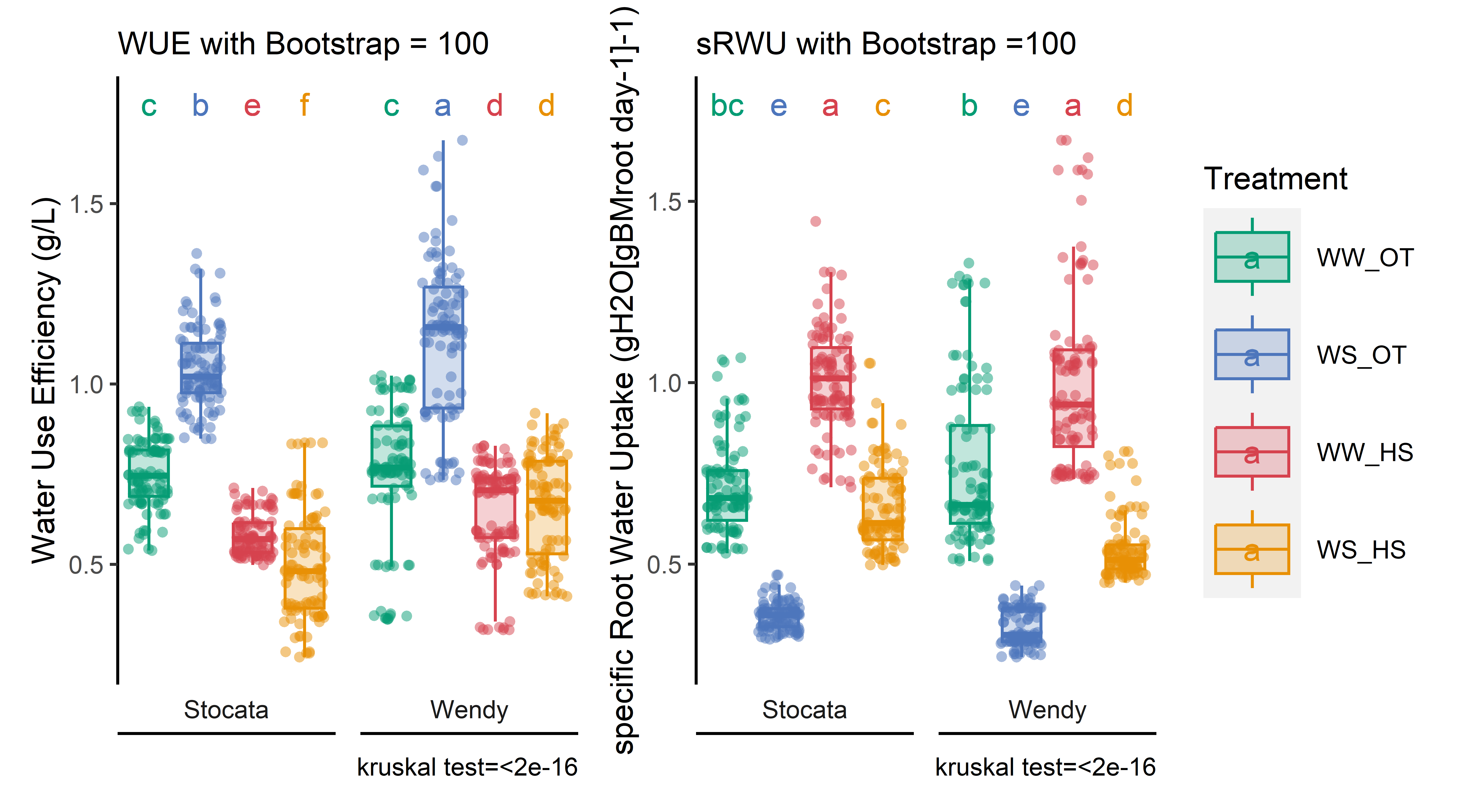```{r}# show tableread.csv(here::here("data/water/weighing_watering_output/WUE_sRWU_Bootstrap.csv")) %>%dplyr::select(condition, WUE,sRWU) %>% dplyr::group_by(condition) %>% dplyr::summarise(across(WUE:sRWU, mean, na.rm =TRUE)) %>%kbl(caption ="WUE and sRWU for eatch condition. Bootstrap = 100", col.names=c("Condition", "WUE (g. L H20-1)","sRWU(gH2O[gBMroot day-1]-1)"), digits =2) %>%kable_paper(full_width = F) %>%column_spec(2, color ="white",background =spec_color(read.csv(here::here("data/water/weighing_watering_output/WUE_sRWU_Bootstrap.csv")) %>%dplyr::group_by(condition) %>% dplyr::summarise(across(WUE:sRWU, mean, na.rm =TRUE)) %>%pull(WUE), end =0.7)) %>%column_spec(3, color ="white",background =spec_color(read.csv(here::here("data/water/weighing_watering_output/WUE_sRWU_Bootstrap.csv")) %>%dplyr::group_by(condition) %>%dplyr::summarise(across(WUE:sRWU, mean, na.rm =TRUE)) %>%pull(sRWU), end =0.7))```## Evapo / Surface```{r , eval=F}sum_evapo_end_and_physio= full_join(read.csv2(here::here("data/water/weighing_watering_output/sum_evapotranspi.csv"), sep=",",dec=".")[-1],read.csv2(here::here("data/physio/global_physio.csv")) %>% dplyr::select(plant_id,plant_num, weight_root, leaf_area,sum_biomass), by="plant_id") %>% mutate(sum_total_evapotranspiration=sum_total_evapotranspiration/2) %>% drop_na(leaf_area,sum_total_evapotranspiration) %>% mutate(evapo_surface=sum_total_evapotranspiration/leaf_area) %>% mutate(water_condition=str_sub(condition, 5, 6)) %>% mutate(heat_condition=str_sub(condition, 8, 9)) %>% mutate(climat_condition=paste0(water_condition, "_", heat_condition)) %>% mutate(condition=factor(condition,levels=c("Sto_WW_OT","Sto_WS_OT","Sto_WW_HS","Sto_WS_HS","Wen_WW_OT","Wen_WS_OT","Wen_WW_HS","Wen_WS_HS"))) %>% mutate(climat_condition=factor(climat_condition,levels=c("WW_OT","WS_OT","WW_HS","WS_HS"))) %>% mutate(genotype=ifelse(str_sub(condition, 1, 3)=="Sto","Stocata","Wendy")) sum_evapo_end_and_physio_H1=sum_evapo_end_and_physio %>% filter(recolte==1)sum_evapo_end_and_physio_H2=sum_evapo_end_and_physio %>% filter(recolte==2)#creation of tablesum_evapo_end_and_physio_H2 %>% dplyr::select(condition, sum_total_evapotranspiration, leaf_area,evapo_surface) %>% dplyr::group_by(condition) %>% dplyr::summarise(across(sum_total_evapotranspiration : evapo_surface, list(mean,sd), na.rm = TRUE)) %>% kbl(caption = "Evapotranspiration by surface of leaf (Mean)", col.names=c("Condition", "Evapotranspiration total during the experiment (mL)", "sd","Leaf area (cm²)", "sd", "Evapo / Leaf surface area (g/cm²)", "sd"), digits = 2) %>% kable_paper(full_width = F)``````{r , eval=F}px_H2=stat_analyse(data =sum_evapo_end_and_physio_H2, column_value = "evapo_surface", category_variables = c("climat_condition"), grp_var = "genotype", control_conditions = c("WW_OT"), biologist_stats = T, strip_normale = F, outlier_show = F, label_outlier = "plant_num", show_plot = T, hex_pallet = climate_pallet, Ylab_i = paste0("Total evapotranspiration \n per leaf area (gH2O/cm²)") )px_H2<-px_H2[["plot"]]+labs(color="Treatment",fill="Treatment")+ theme(axis.title.x=element_blank(), axis.text.x=element_blank(), panel.grid.major = element_blank(), panel.grid.minor = element_blank(), axis.ticks.x = element_blank() )px_H1=stat_analyse(data =sum_evapo_end_and_physio_H1 %>% mutate(genotype=as.factor(genotype)) %>% filter(plant_num!=2), # leaf area is wrong (not well developed) column_value = "evapo_surface", category_variables = "genotype", control_conditions = "", biologist_stats = T, strip_normale = F, outlier_show = F, label_outlier = "plant_num", show_plot = T, hex_pallet = climate_pallet, Ylab_i = paste0("Total evapotranspiration \n per leaf area (gH2O/cm²)") )px_H1<-px_H1[["plot"]]+labs(color="Treatment",fill="Treatment")+ theme(axis.title.x=element_blank(), axis.text.x=element_blank(), panel.grid.major = element_blank(), panel.grid.minor = element_blank(), axis.ticks.x = element_blank() )combined_plot<-(px_H1+px_H2) #+ plot_layout(guides = 'collect')# export figurepng(here::here(paste0("report/water/plot/evapo_leaf.png")), width = 18, height = 10, units = 'cm', res = 900)combined_plotdev.off()``````{r , eval=F}p_licor=stat_analyse(data =read.csv2(here::here("data/physio/global_physio.csv")) %>% dplyr::select(plant_num,condition,genotype,Trmmol) %>% mutate(water_condition=str_sub(condition, 5, 6)) %>% mutate(heat_condition=str_sub(condition, 8, 9)) %>% mutate(climat_condition=paste0(water_condition, "_", heat_condition)) %>% mutate(condition=factor(condition,levels=c("Sto_WW_OT","Sto_WS_OT","Sto_WW_HS","Sto_WS_HS","Wen_WW_OT","Wen_WS_OT","Wen_WW_HS","Wen_WS_HS"))) %>% mutate(climat_condition=factor(climat_condition,levels=c("WW_OT","WS_OT","WW_HS","WS_HS"))) %>% drop_na(Trmmol), column_value = "Trmmol", category_variables = c("climat_condition"), grp_var = "genotype", control_conditions = c("WW_OT"), biologist_stats = T, strip_normale = F, outlier_show = F, label_outlier = "plant_num", show_plot = T, hex_pallet = climate_pallet, Ylab_i = paste0("Transpiration rate (mmol H2O.m-2.s-1)") )p_licor<-p_licor[["plot"]]+labs(color="Treatment",fill="Treatment")+ theme(axis.title.x=element_blank(), axis.text.x=element_blank(), panel.grid.major = element_blank(), panel.grid.minor = element_blank(), axis.ticks.x = element_blank() )# export figurepng(here::here(paste0("report/water/plot/Transpiration_rate.png")), width = 14, height = 8, units = 'cm', res = 900)p_licordev.off()# for humidity close to the leaves ###################p_H2OS=stat_analyse(data =read.csv2(here::here("data/physio/global_physio.csv")) %>% dplyr::select(plant_num,condition,genotype,H2OS) %>% mutate(water_condition=str_sub(condition, 5, 6)) %>% mutate(heat_condition=str_sub(condition, 8, 9)) %>% mutate(climat_condition=paste0(water_condition, "_", heat_condition)) %>% mutate(condition=factor(condition,levels=c("Sto_WW_OT","Sto_WS_OT","Sto_WW_HS","Sto_WS_HS","Wen_WW_OT","Wen_WS_OT","Wen_WW_HS","Wen_WS_HS"))) %>% mutate(climat_condition=factor(climat_condition,levels=c("WW_OT","WS_OT","WW_HS","WS_HS"))) %>% drop_na(H2OS), column_value = "H2OS", category_variables = c("climat_condition"), grp_var = "genotype", control_conditions = c("WW_OT"), biologist_stats = T, strip_normale = F, outlier_show = F, label_outlier = "plant_num", show_plot = T, hex_pallet = climate_pallet, Ylab_i = paste0("Moisture on leaf surface (%)") )p_H2OS<-p_H2OS[["plot"]]+labs(color="Treatment",fill="Treatment")+ theme(axis.title.x=element_blank(), axis.text.x=element_blank(), panel.grid.major = element_blank(), panel.grid.minor = element_blank(), axis.ticks.x = element_blank() )# for temperature of the leaves ###################p_Tleaf=stat_analyse(data =read.csv2(here::here("data/physio/global_physio.csv")) %>% dplyr::select(plant_num,condition,genotype,Tleaf) %>% mutate(water_condition=str_sub(condition, 5, 6)) %>% mutate(heat_condition=str_sub(condition, 8, 9)) %>% mutate(climat_condition=paste0(water_condition, "_", heat_condition)) %>% mutate(condition=factor(condition,levels=c("Sto_WW_OT","Sto_WS_OT","Sto_WW_HS","Sto_WS_HS","Wen_WW_OT","Wen_WS_OT","Wen_WW_HS","Wen_WS_HS"))) %>% mutate(climat_condition=factor(climat_condition,levels=c("WW_OT","WS_OT","WW_HS","WS_HS"))) %>% drop_na(Tleaf), column_value = "Tleaf", category_variables = c("climat_condition"), grp_var = "genotype", control_conditions = c("WW_OT"), biologist_stats = T, strip_normale = F, outlier_show = F, label_outlier = "plant_num", show_plot = T, hex_pallet = climate_pallet, Ylab_i = paste0("Leaf surface temperature (°C)") )p_Tleaf<-p_Tleaf[["plot"]]+labs(color="Treatment",fill="Treatment")+ theme(axis.title.x=element_blank(), axis.text.x=element_blank(), panel.grid.major = element_blank(), panel.grid.minor = element_blank(), axis.ticks.x = element_blank() )# for stomatac conductance of the leaves ###################p_Gs=stat_analyse(data =read.csv2(here::here("data/physio/global_physio.csv")) %>% dplyr::select(plant_num,condition,genotype,Cond) %>% mutate(water_condition=str_sub(condition, 5, 6)) %>% mutate(heat_condition=str_sub(condition, 8, 9)) %>% mutate(climat_condition=paste0(water_condition, "_", heat_condition)) %>% mutate(condition=factor(condition,levels=c("Sto_WW_OT","Sto_WS_OT","Sto_WW_HS","Sto_WS_HS","Wen_WW_OT","Wen_WS_OT","Wen_WW_HS","Wen_WS_HS"))) %>% mutate(climat_condition=factor(climat_condition,levels=c("WW_OT","WS_OT","WW_HS","WS_HS"))) %>% drop_na(Cond), column_value = "Cond", category_variables = c("climat_condition"), grp_var = "genotype", control_conditions = c("WW_OT"), biologist_stats = T, strip_normale = F, outlier_show = F, label_outlier = "plant_num", show_plot = T, hex_pallet = climate_pallet, Ylab_i = expression(G[s] ~ "(" * mol ~ H[2]*O ~ m^{-2} ~ s^{-1} * ")"), )p_Gs<-p_Gs[["plot"]]+labs(color="Treatment",fill="Treatment")+ theme(axis.title.x=element_blank(), axis.text.x=element_blank(), panel.grid.major = element_blank(), panel.grid.minor = element_blank(), axis.ticks.x = element_blank() )# export figurepng(here::here(paste0("report/water/plot/Transpiration_rate.png")), width = 14, height = 8, units = 'cm', res = 900)p_licordev.off()png(here::here(paste0("report/water/plot/H2OS.png")), width = 14, height = 8, units = 'cm', res = 900)p_H2OSdev.off()png(here::here(paste0("report/water/plot/Tleaf.png")), width = 12, height = 8, units = 'cm', res = 900)p_Tleafdev.off()png(here::here(paste0("report/water/plot/Gs.png")), width = 12, height = 8, units = 'cm', res = 900)p_Gsdev.off()```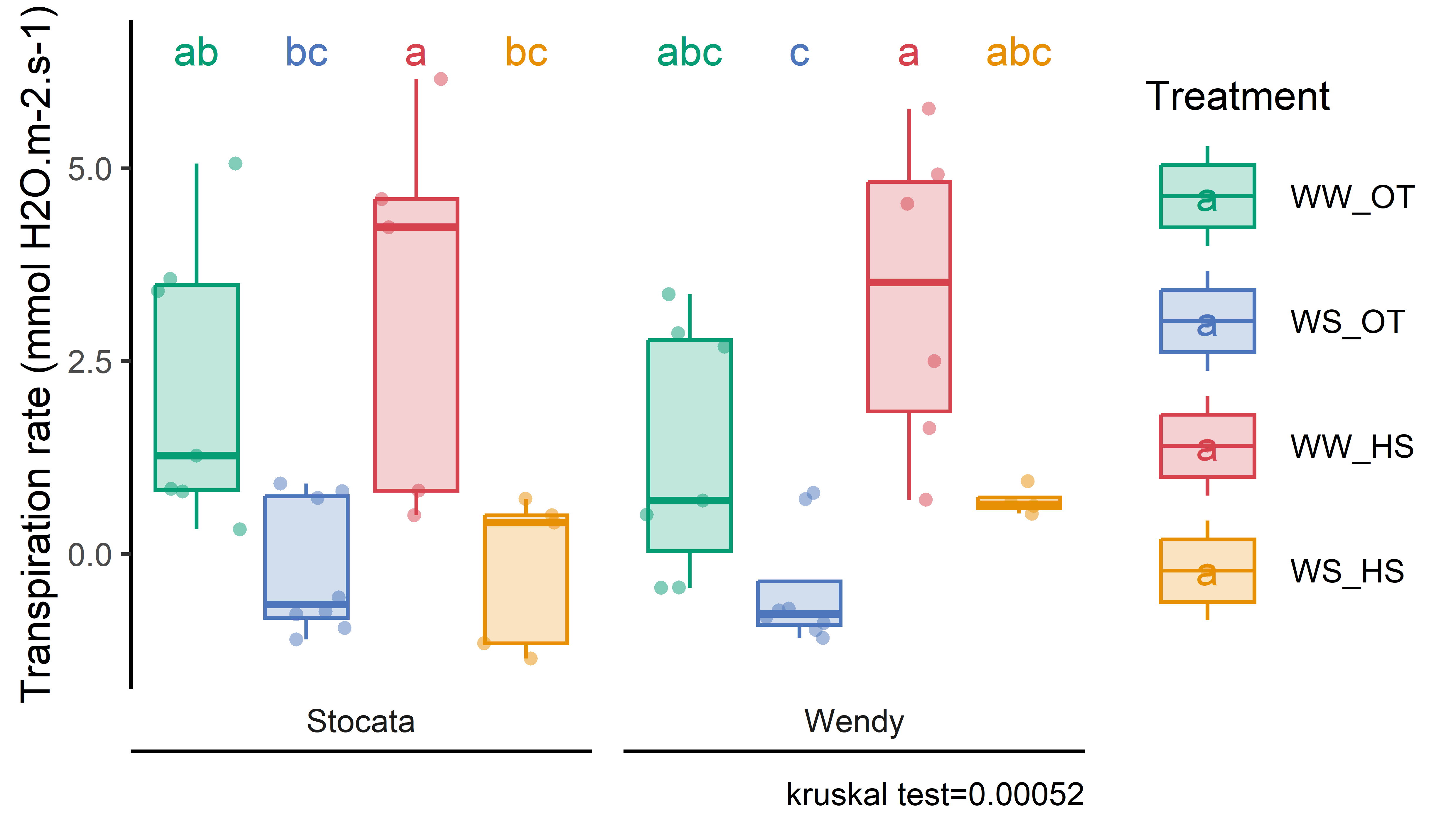## Evaporation one days befor second harvest```{r}# calculdf_evapo_biomass<-read.csv(here::here("data/water/weighing_watering_output/df_evapo3.csv"))[-1] %>%arrange(next_weight) %>%filter(resultdate=="2021-10-11") %>%filter(taskid %in%c(28697, 28699)) %>%drop_na(leaf_area) %>%mutate(diff_resultdate_time_h=diff_resultdate_time/60) %>%mutate(leaf_area_m=leaf_area/10000) %>%mutate(transpiPlante_g_h=evapotranspiration/(2*diff_resultdate_time/60)) %>%mutate(TR_g_m2_s=transpiPlante_g_h/(leaf_area_m*3600)) %>%mutate(TR_mmol_m2_s=TR_g_m2_s*10^3/18.015) %>%distinct(plant_num, .keep_all =TRUE)# exportwrite.csv(df_evapo_biomass, here::here("data/water/weighing_watering_output/transpiration_rate_20231011.csv"))# creation tabledf_evapo_biomass_mean = df_evapo_biomass %>%dplyr::select(condition, transpiPlante_g_h, leaf_area,diff_resultdate_time,TR_mmol_m2_s) %>% dplyr::group_by(condition) %>% dplyr::summarise(across(transpiPlante_g_h : TR_mmol_m2_s, list(mean,sd), na.rm =TRUE))df_evapo_biomass_mean %>%kbl(caption ="Evapotranspiration by surface of leaf between two measure (Mean)", col.names=c("Condition", "Plant transpiration (g/h)", "sd","Leaf area (cm²)", "sd","time between two weighings (min)","sd", "Transpiration rate (mmol m-2 s-1", "sd"), digits =2) %>%kable_paper(full_width = F) %>%column_spec(8, color ="white",background =spec_color(df_evapo_biomass_mean %>%pull(TR_mmol_m2_s_1), end =0.7)) ``````{r, eval=F}px=stat_analyse(data =df_evapo_biomass %>% #mutate(heat_condition=str_sub(condition, 8, 9)) %>% mutate(climat_condition=paste0(water_condition, "_", heat_condition)) %>% #mutate(condition=factor(condition,levels=c("Sto_WW_OT","Sto_WS_OT","Sto_WW_HS","Sto_WS_HS","Wen_WW_OT","Wen_WS_OT","Wen_WW_HS","Wen_WS_HS"))) %>% mutate(climat_condition=factor(climat_condition,levels=c("WW_OT","WS_OT","WW_HS","WS_HS"))) %>% drop_na(TR_mmol_m2_s), column_value = "TR_mmol_m2_s", category_variables = c("climat_condition"), grp_var = "genotype", control_conditions = c("WW_OT"), biologist_stats = T, strip_normale = F, outlier_show = F, label_outlier = "plant_num", show_plot = T, hex_pallet = climate_pallet, Ylab_i = paste0("Evapotranspiration during licore measure \n per leaf area (mmol.m-2.s-1)") )px<-px[["plot"]]+labs(color="Treatment",fill="Treatment")+ theme(axis.title.x=element_blank(), axis.text.x=element_blank(), panel.grid.major = element_blank(), panel.grid.minor = element_blank(), axis.ticks.x = element_blank() )# export figurepng(here::here(paste0("report/water/plot/Transpiration_rate_20211011.png")), width = 14, height = 10, units = 'cm', res = 900)pxdev.off()```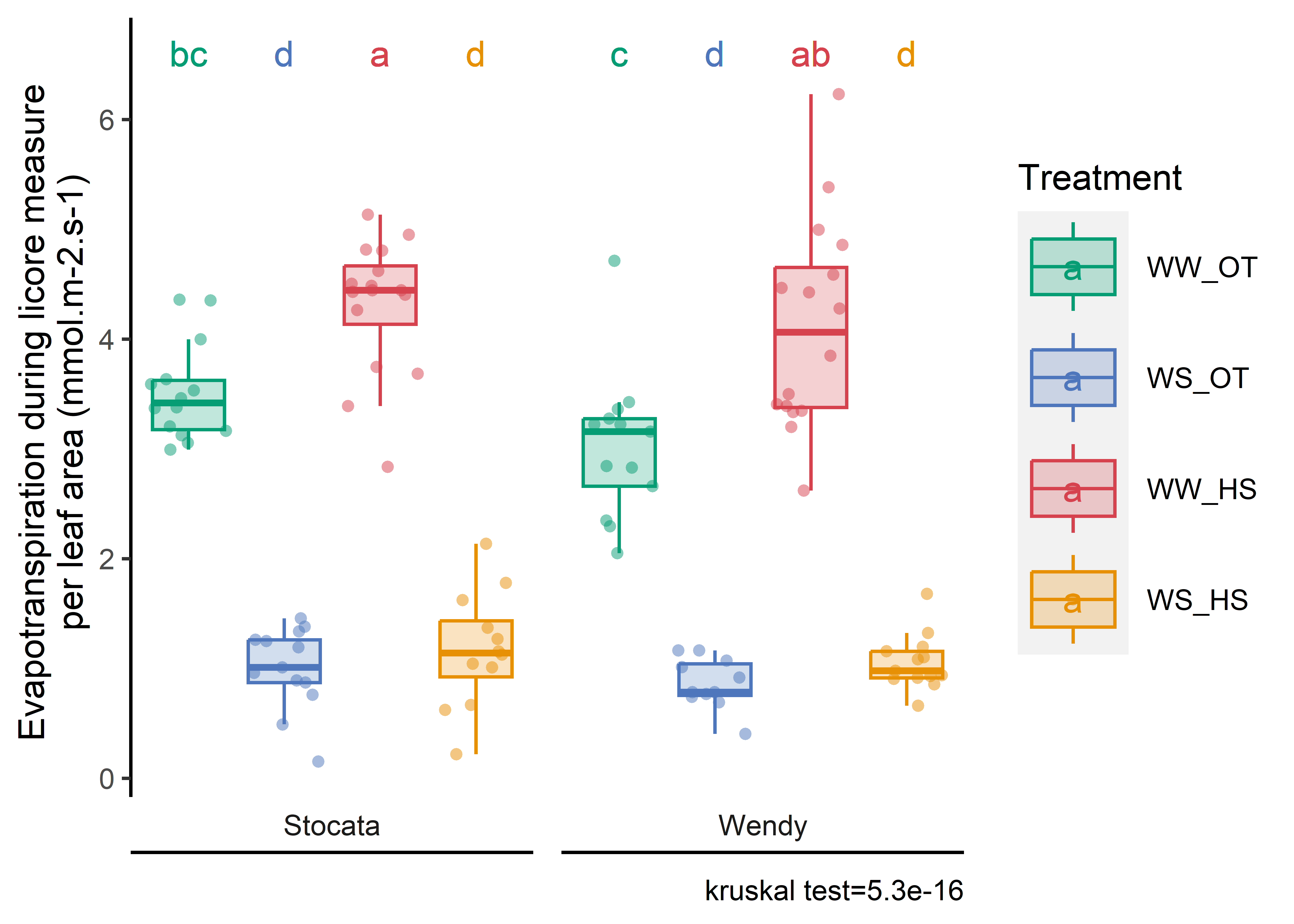<details><summary style="color: #007bff;">Bonnus: Draft of some statistics</summary>```{r, eval=F}test=df_compile_sRWU %>% drop_na(sRWU) %>% #filter(climat_condition=="WW_OT") %>% t_test(sRWU ~ condition,p.adjust.method = "BH") %>% add_significance()test=df_compile %>% drop_na(WUE) %>% #filter(climat_condition=="WW_OT") %>% t_test(WUE ~ condition,p.adjust.method = "BH") %>% add_significance()``````{r,eval=F}df_physio_s=df_compile %>% drop_na(WUE) %>% #filter(genotype=="Stocata") %>% #filter(condition%in% c("Sto_WW_HS","Wen_WW_HS")) %>% dplyr::group_by(condition) %>% dplyr::summarise(Mean=mean(WUE))(df_physio_s$Mean[4]-df_physio_s$Mean[8])/df_physio_s$Mean[8]```</details>


